
5.2 Intermediate Table Skills
Learning Objectives
- Sort table data.
- Custom Sort table data.
- Apply Custom List sort options.
- Filter table data using criteria filters.
INTERMEDIATE TABLE SKILLS
SORT, FILTER, AND ANALYZE DATA
SORTING
Sorting is one of the most common tools for data management. By arranging data sequentially the information becomes more meaningful. Arranging records in a specific sequence is called sorting. If you sort by one column this is considered a single sort. If you need to sort by more than one column, this is considered a custom sort.
The field or fields you select to sort are called sort keys. In Excel, you can sort your table by ascending or descending order. Data in ascending order appears lowest to highest, earliest to most recent, or alphabetically from A to Z. Data in descending order in arranged by highest to lowest, most recent to earliest, or alphabetically from Z to A.
Excel will sort a range of data that is not in a table. However, when working with large sets of information it is wise to make the data a table for integrity. Excel locks the row of information creating a record, thus when sorted, the record remains intact, just reorganized. For example, when you sort the table by last name, all of the records in each row move together. It is always a good idea to save a copy of your worksheet before applying sorts.
There are multiple places you can find and use sorting tools:
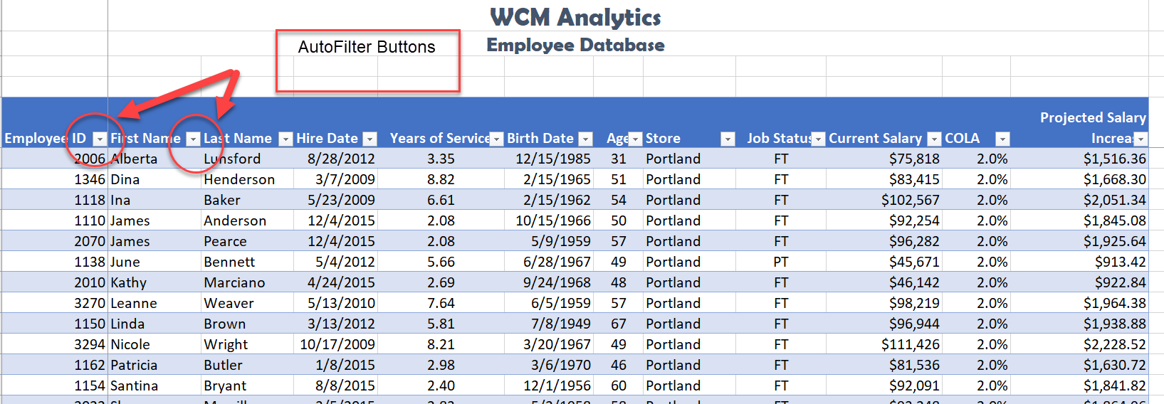
- When you first create a table, Excel automatically enables AutoFilter buttons; a tool used to sort, query, and filter the records in a table. The filter buttons appear to the right of the column headings. When you click the filter button sorting options appear on the menu options.
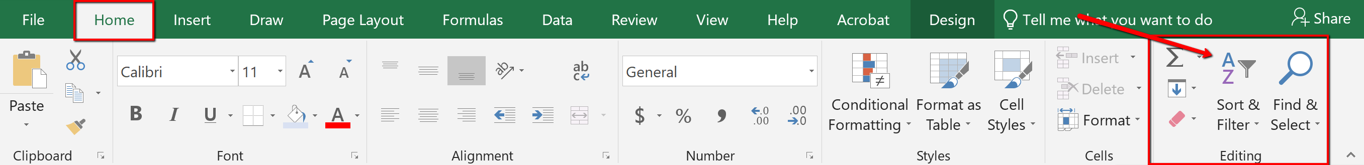
- From the Home tab, in the Editing group, click the ‘Sort & Filter’ button, and then click one of the sorting options on the Sort & Filter menu.
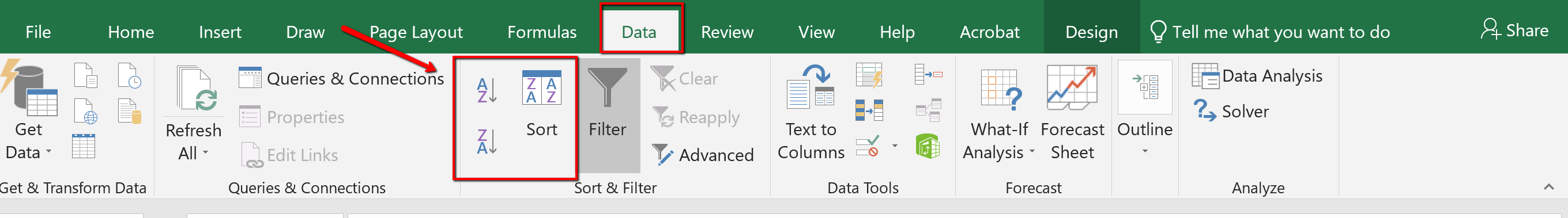
- From the Data tab, use the ‘Sort A to Z’ or ‘Sort Z to A’ buttons or for multiple levels select the Sort button to open the Custom Sort dialogue.
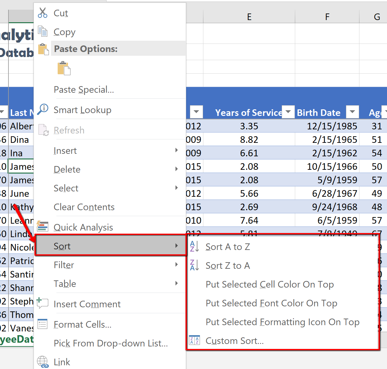
- Right-click anywhere in a table and then point to Sort on the shortcut menu to display the Sort sub-menu.
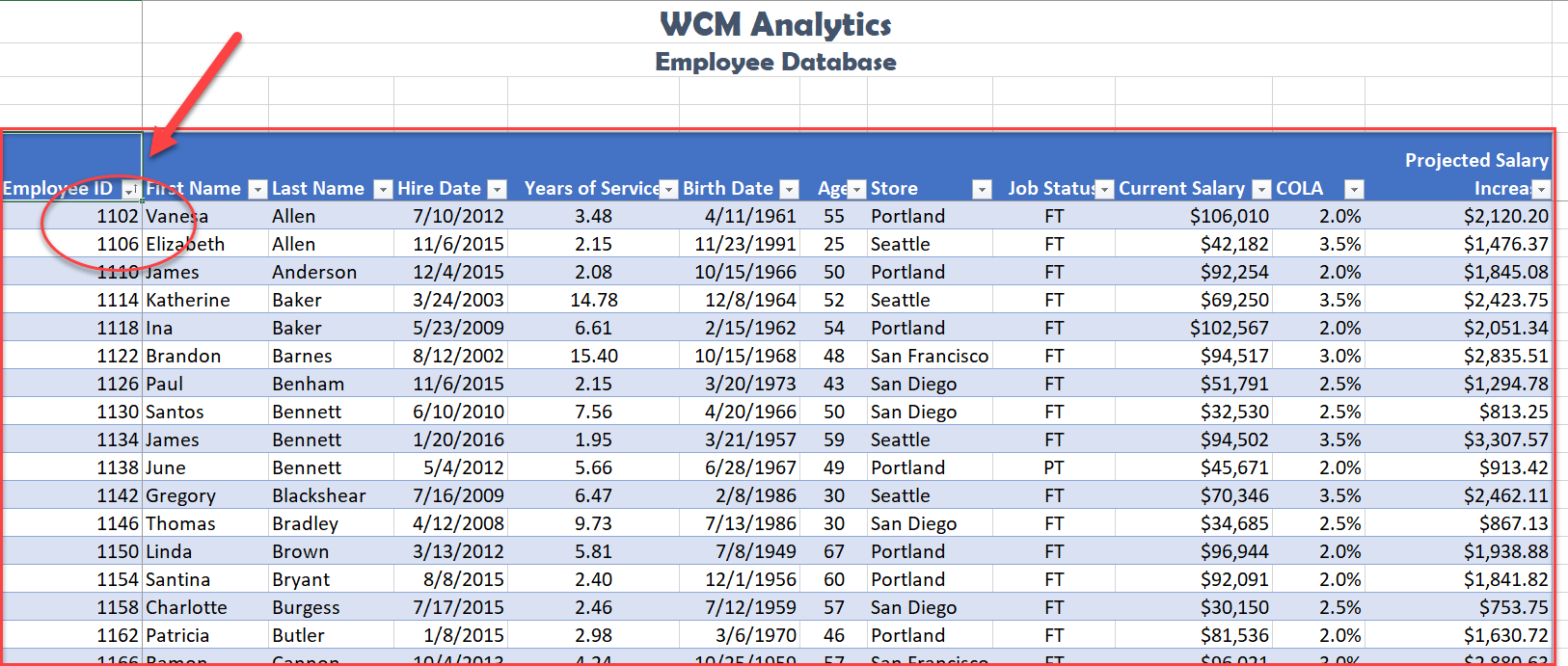
Complete a single level sort by following the steps:
1. In the EmployeeID heading, click the filter button.
2. Choose to Sort Smallest to Largest.
![]() Mac Users: Click the A-Z Ascending button
Mac Users: Click the A-Z Ascending button ![]()
Notice Excel arranges in chronological order all the employee data based on the EmployeeID number, however keeping each record together. You will also notice the filter button now displays an up arrow denoting an ascending sort.
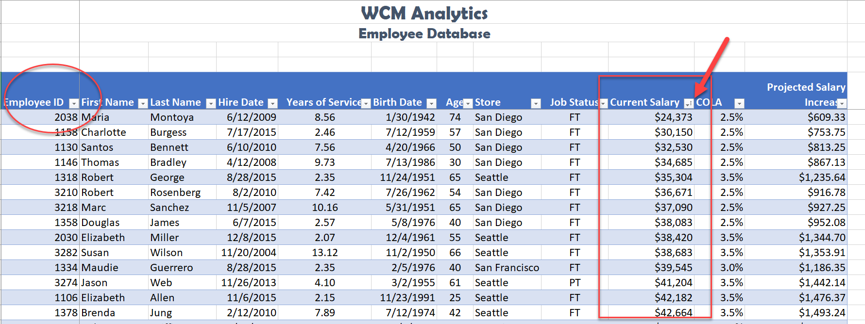
The following steps will sort the records in descending order by Current Salary using the ‘Sort Largest to Smallest’ option form the filter button.
1. Click the filter button located in the Current Salary heading.
2. Choose Sort Largest to Smallest option from the menu.
![]() Mac Users: click the “Descending” button
Mac Users: click the “Descending” button
Notice the original sort has been overridden, and the information is now organized based on the largest Current Salary. You will see the small arrow on the EmployeeID filter is gone, and an arrow pointing down for Descending Order is visible on the Current Salary filter button.
Skill Refreshed
Sort a Column
- Click on the filter Click arrow to the right of the header in the column you want to sort.
- Click on the choice AZ↑ or ZA↓ to sort your data by that column.
CUSTOM SORT
When you need to sort by more than one level, you must use the Custom Sort option. Complete the following steps to organize the data by Store, Last Name, Current Salary, all in Ascending Order (A-Z).
1. Select the Data tab, and click the Sort button. Notice the last column sorted by is listed. Change the column heading name by dropping down the Sort by menu and select Store.
2. Click Add Level.
![]() Mac Users: click the + symbol
Mac Users: click the + symbol ![]()
3. Click the down arrow in the Then by section, and choose the column heading names as shown below in Figure 5.29. Note to click Add Level to add the next column heading. The order you select the headings will determine how the table information is sorted.
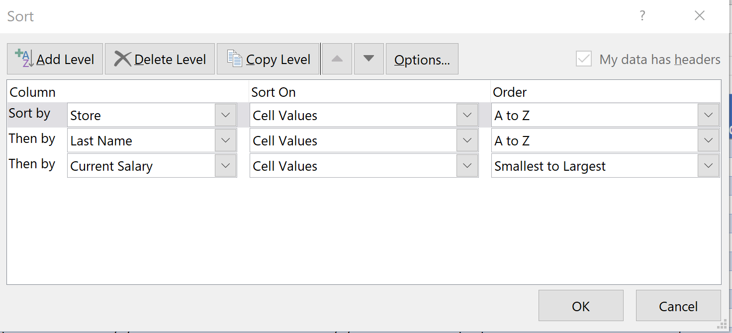
4. Once you select to Sort by column headings, choose the Order by selecting to sort in ascending order (A-Z) for the Store and Last name fields, and Smallest to Largest, for the Current Salary field.
5. Click OK.
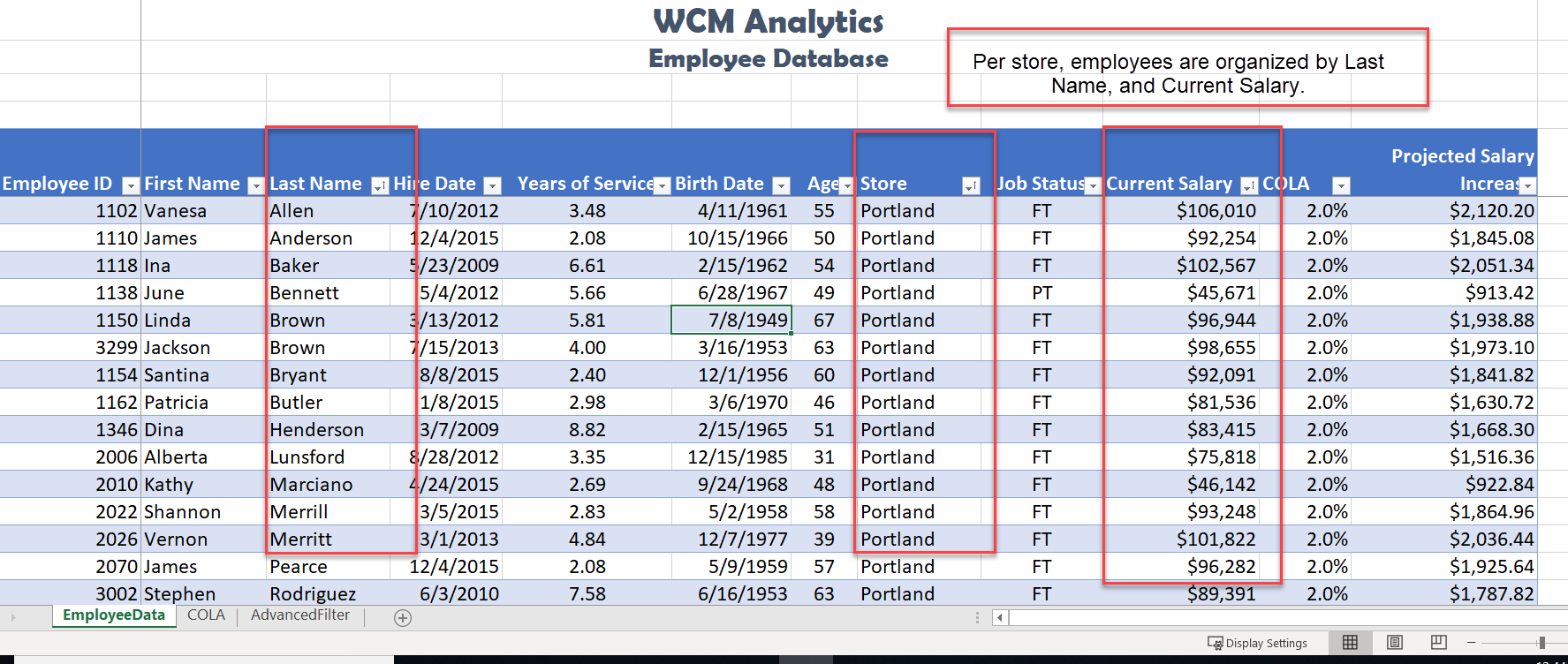
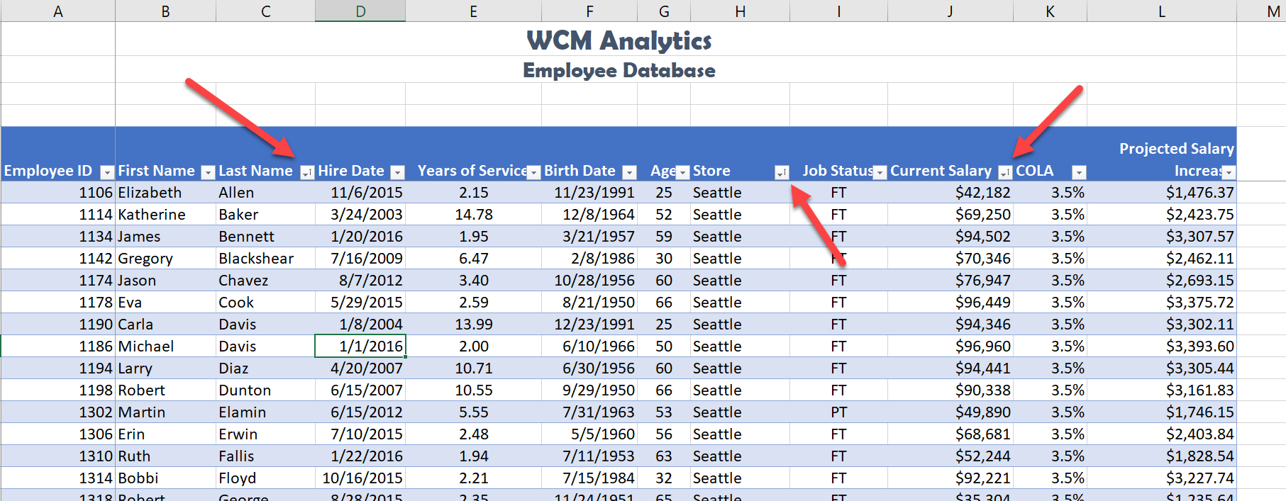
Notice the information is now sorted by three levels, per Store, each employee is organized by Last Name, and Current Salary in ascending order (smallest to largest). Each of the filter buttons indicates the sort with the up arrow.
Skill Refresher
Custom Sort (Multiple Level Sort)
- Select the Data tab, and click the Sort button.
- Choose Add Level.
- Click the down arrow in the Column field and choose the column heading to sort by.
- Repeat the above steps to add another level and select the next column heading to sort by.
- The order you select the headings will determine how the table information is sorted.
CUSTOM LIST SORT
When sorting you can create custom lists that allow sorting by characteristics that do not sort alphabetically. Example, text items such as high, medium, and low—or S, M, L, XL. Dates commonly require custom lists so you can vary in the way data is sorted by days of the week or months of the year.
In our case, we want to create a custom list that sorts our stores, which is not, in ascending or descending order. The human resources office likes to order the stores based on the location size. The company headquarters is in Seattle and employs the most people. The next biggest location is San Diego etc. Follow the below steps to create a custom list ordering the stores as shown below:
Seattle
San Diego
Portland
San Francisco
![]() Mac Users: The steps to create a custom sort list are different for Excel for Mac. Please skip the below steps and follow the alternate steps below Figure 5.34.
Mac Users: The steps to create a custom sort list are different for Excel for Mac. Please skip the below steps and follow the alternate steps below Figure 5.34.
Follow the below steps to create a custom list ordering:
- While clicked in the table, choose the Data tab and click the Sort button.
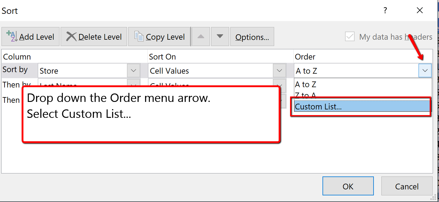
- In the Sort by row, click the drop-down menu in the Order Column for the Store heading. Choose Custom List.
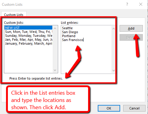
3. Click in the List entries: box and type Seattle, and press enter. Type the remainder of the locations shown in Figure 5.32, pressing enter after each store location typed. Once all locations are entered, click Add. Then choose Ok.
4. You will see the Order of the Store sort update. Click OK to close the Sort dialogue box.
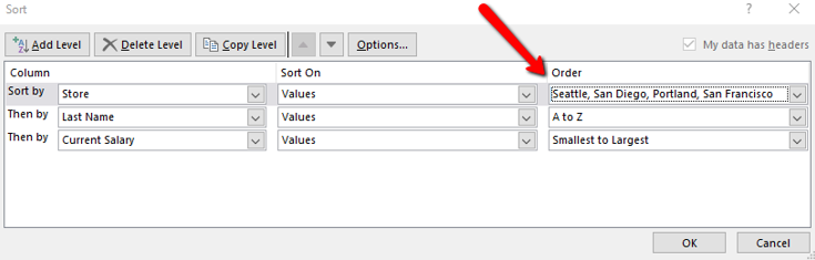
The custom sort is applied and the table is now sorted by Store, using the custom order, then the Last Name of the employee and then by the Current Salary column.
![]() Mac Users alternate steps for creating a custom sort list:
Mac Users alternate steps for creating a custom sort list:
- Click the Excel menu option and choose Preferences
- Click on the Custom List button
- Type the list of cities in the “List entries” box as shown in Figure 5.32 above then click the Add button and close the Custom List dialog box
- Click anywhere in the table, and then click the Data tab and click the Sort button
- Click the drop-down menu in the Order Column for the Store heading. Choose Custom List
- Click on the custom list of cities that you just created and then click the OK button twice
- The custom sort is applied and the table is now sorted by Store, using the custom order, then the Last Name of the employee and then by the Current Salary column. See Figure 5.34 above.
Custom List Sort
- Select the Data tab, and click the Sort button.
- Click the drop-down menu in the Order Column of the field needing a custom list created.
- Choose Custom List.
- Click in the List entries box and type the custom list desired.
- Then click Add.
- Click Ok.
FILTER DATA
If your worksheet contains a lot of data, it can be difficult to find information quickly. Applying Filters is an efficient and effective way to only show the information needed. Typically when filtering you are searching the data for specific information. Generally speaking, you are searching the data based on a question, or in other words, querying the data, and returning only the information that satisfies the question. The process of filtering records based on one or more filter criteria is called a query. Filtering data hides the rows whose values do not match the search criteria. The information that does not display is not deleted, it is just hidden, and will be redisplayed by removing the filter or applying a new filter.
Like sorting, Filter options are located in the filter button alongside each field name. By clicking the filter button, you can choose which values in that field to display, hiding the rows or records that do not match that value. The filter lets you choose to display only those records that meet specified criteria such as color, number, or text. In this situation, criteria is defined as; a logical rule by which data is tested and chosen.
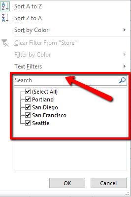
For example, you can filter the table to display a specific name or item by typing it in a Search box. The name you selected acts as the criterion for filtering the table, which results in Excel displaying only those records that match the criterion. The selected checkboxes indicate which items will appear in the table. By default, all of the items are selected. If you deselect an item from the filter menu, it is removed from the filter criterion. Excel will not display any record that contains the unchecked item. As with the previous sort techniques, you can include more than one column when you filter by clicking a second filter button and making choices. After you filter data, you can copy, find, edit, format, chart, or print the filtered data without rearranging or moving it.
Complete the following steps and filter data according to each query.
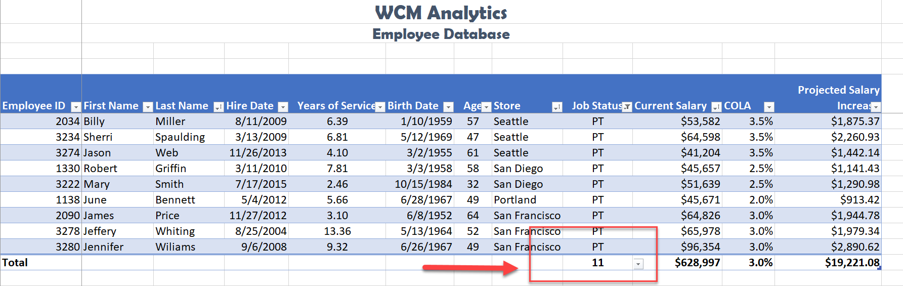
How many employees are at a Part-Time (PT) status?
- Click the filter button on the Job Status column heading.
- Click Select All, to deselect options.
- Click the PT box to only display the part-time employees.
- From the total row, in cell I108, choose the Count function count the number of employees at a PT status.
The answer to the question is there are currently are 11 employees at a PT time status. The total row will display the part-time total current salaries, and what the projected salary increase for part-time help will be after COLA adjustments.
USING CRITERIA FILTERS
The filters created are limited to selecting records for fields matching a specific value or set of values. For more general criteria, you can use criteria filters, which are expression involving dates and times, numeric values, and text strings. Excel will identify what criteria filter to display based on the information in the column. For example, you can filter the employee data to show only those employees hired within a specific date range. Notice the criteria filter changes to Date Filters. If we were looking at the Current Salary column, the filter would be a Numbers Filter.
Using criteria filters, follow the below steps to search for employees who have been with the company for a specific time period.
Identify employees who have been with the company between 2013-2016.
1. While clicked in the table, clear any sort or filter applied by clicking the Data tab. In the Sort & Filter group choose the Clear button. ![]()
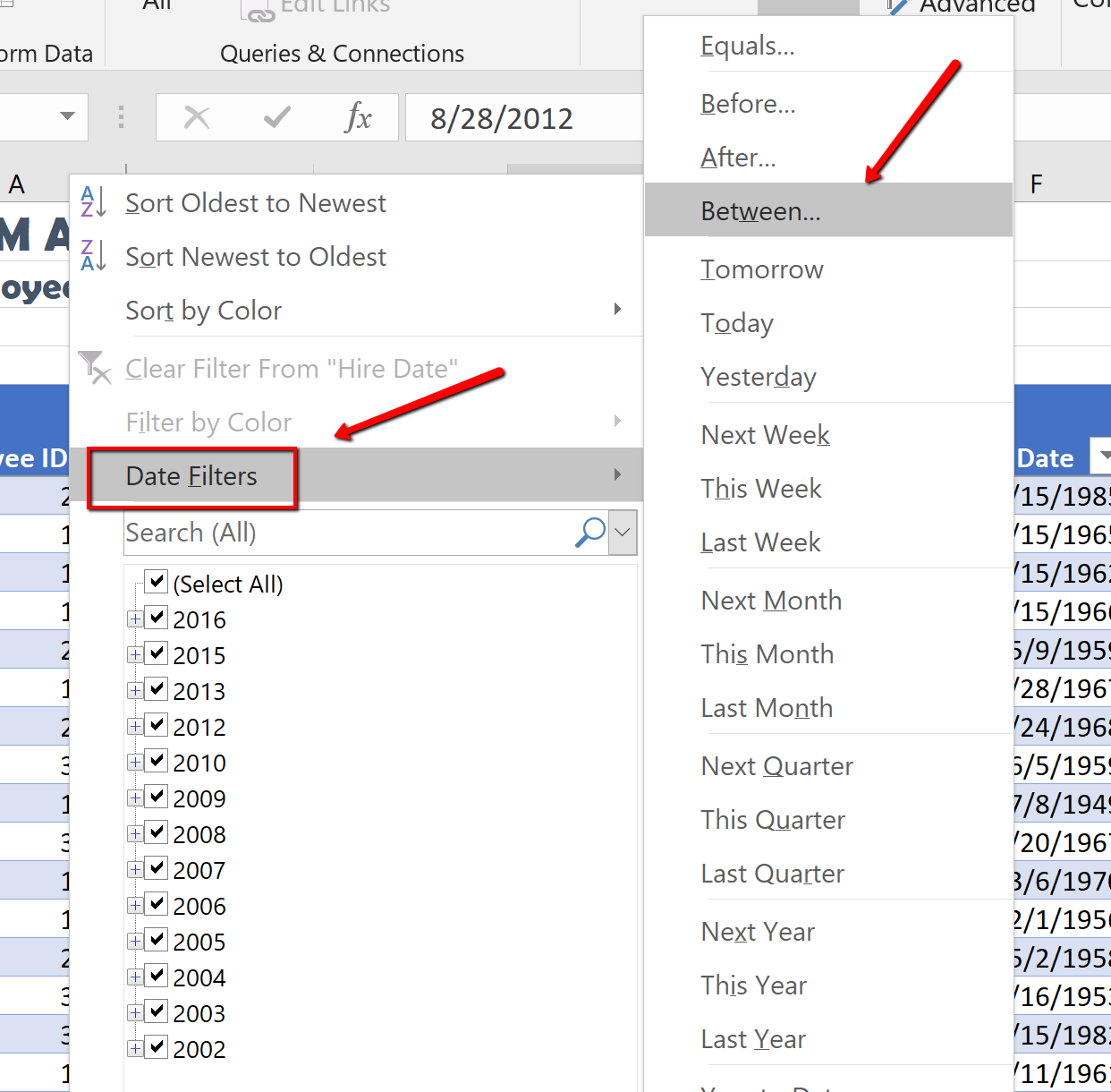
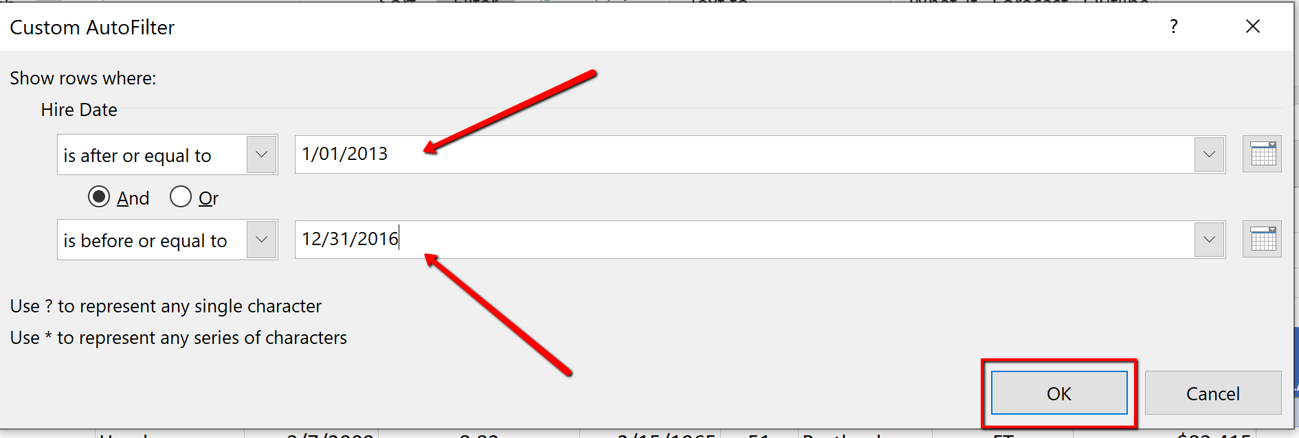
2. Click the Filter button in the Hire Date column. Select Date Filters, and choose the Between criteria.
![]() Mac Users: uncheck the Select All checkbox before choosing the Between option.
Mac Users: uncheck the Select All checkbox before choosing the Between option.
3. Search for employees with a hire date between 2013, and 2016. In the “is after or equal to” section type 1/01/2013, and typing in the “is before or equal to” section type 12/31/2016. Then click OK.
![]() Mac Users: Excel for Mac sections simply say “After” and “Before”
Mac Users: Excel for Mac sections simply say “After” and “Before”
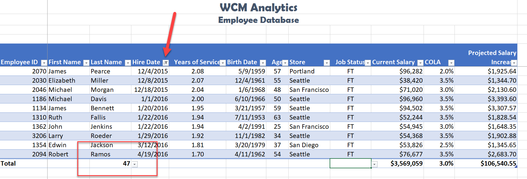
4. Sort the filtered table from Oldest to Newest by Date Hired.
5. In the total row section, count the last name names of the employees by applying the count function in cell B108.
6. In the total row, select cell I108, and choose None to turn off the count function in the Job Status Column.
Notice the table total row show 47 employees hired between the specified dates. These employees will be evaluated for a COLA adjustment.
Notice the filter button displays a filter symbol and an up arrow indicating the column is filtered and sorted in ascending order.
SLICERS
Another way to filter an Excel table is with slicers. Slicers, generally speaking, are visual filter buttons you can click to filter the table data. Slicers show the current filtered category, which makes it easy to understand what exactly is displayed. For example, a slicer for the Store field would have buttons for the Seattle, San Diego, Portland, and San Francisco locations.
When slicer buttons are selected, the data is filtered to show only those records that match the criteria. Multiple buttons can be selected at the same time, and a table can have multiple slicers, each linked to a different field. When multiple slicers are used, Excel uses the AND logical operator so filtered records must meet all of the criteria indicated in the slicer. When selecting multiple buttons in a Slicer, use the shift key to select adjacent field names. If the field names are not adjacent, use the non-adjacent selection method, pressing the CTL button, and selecting the field names needed.
Follow the below steps to filter the table using visual Slicer buttons.
1. Click in the table area. From the Data tab, choose Clear to remove the current sort and filter applied to the data.
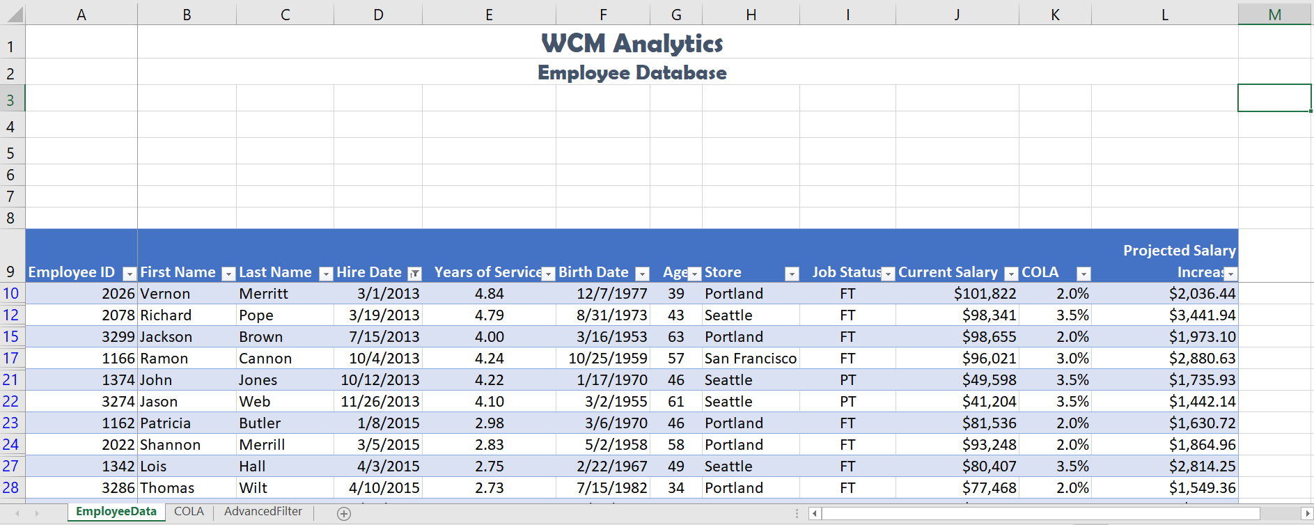
2. To make room for the Slicer buttons at the top of the table, we will add 4 rows between the title and the table area. Right-click cell A3. Choose Insert. Select Entire Row. Repeat these steps until the table heading starts in row A9.
![]() Mac users should hold down CTRL key and click cell A3. Then repeat until the table heading starts in row A9.
Mac users should hold down CTRL key and click cell A3. Then repeat until the table heading starts in row A9.
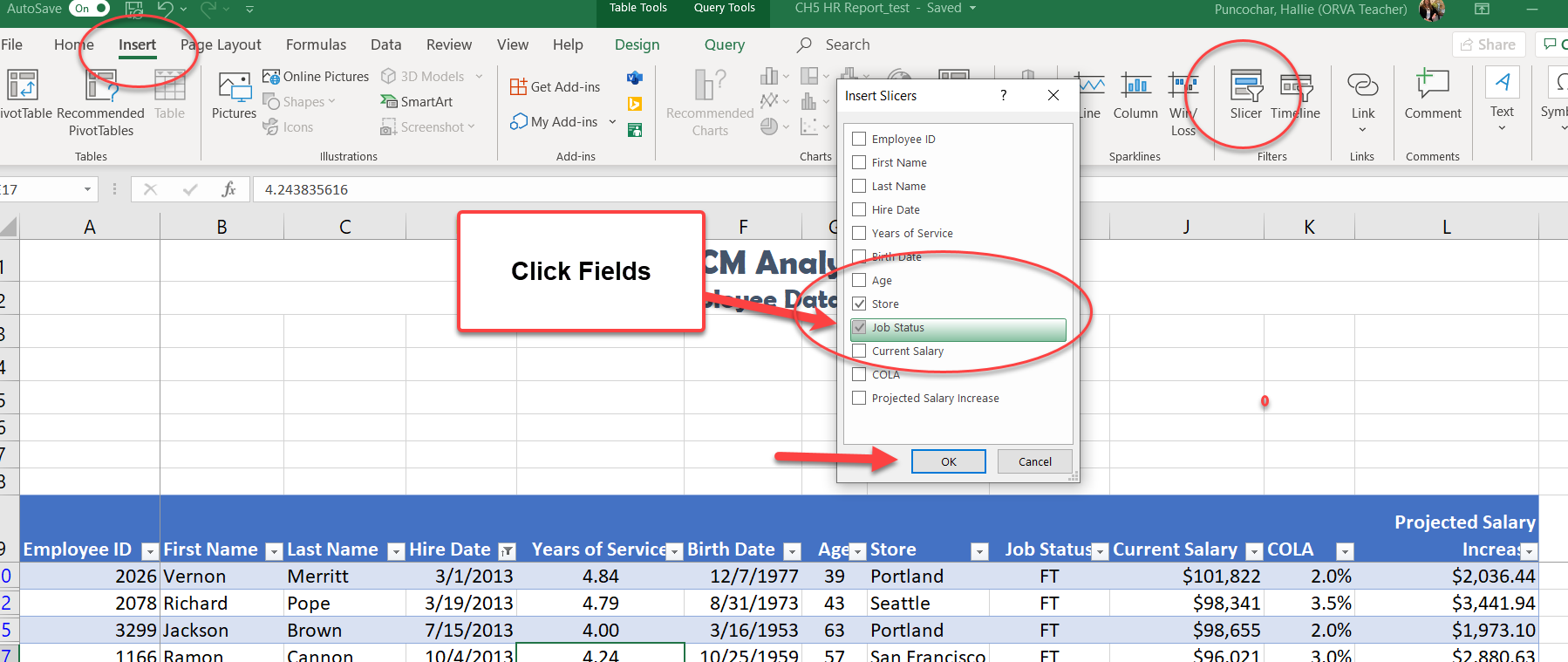
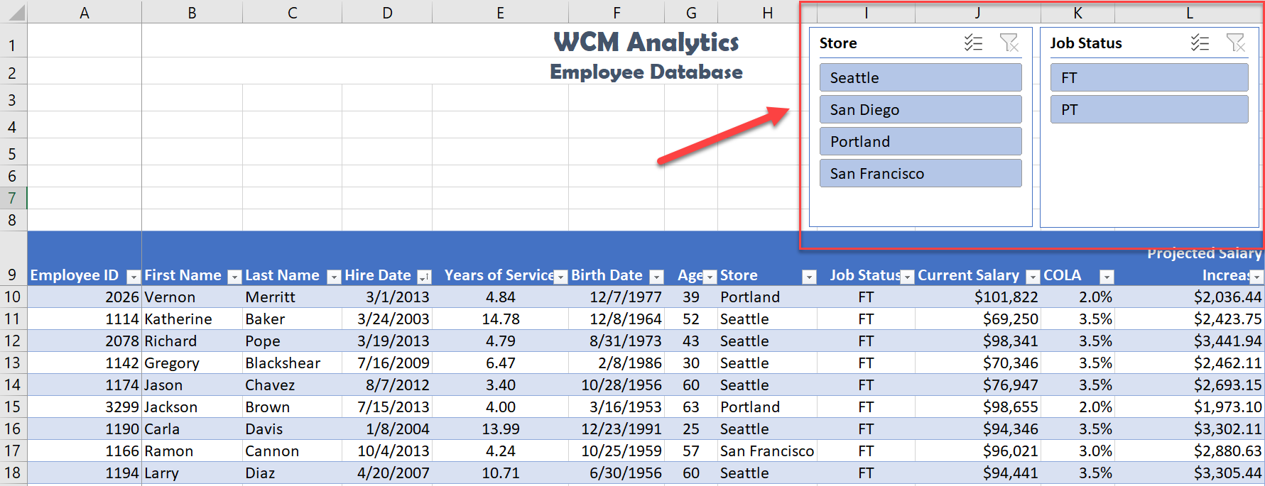
3. Click back into the table area. Choose the Insert tab. Click Slicer. When the Insert Slicers dialogue box opens, click the Store and Job Status field names to display as slicers. Click OK.
4. Move, and re-size the Slicer boxes to fit in the approximate area of I1:J8 and K1:L8. Make sure the buttons remain visible. Below is a visual example.
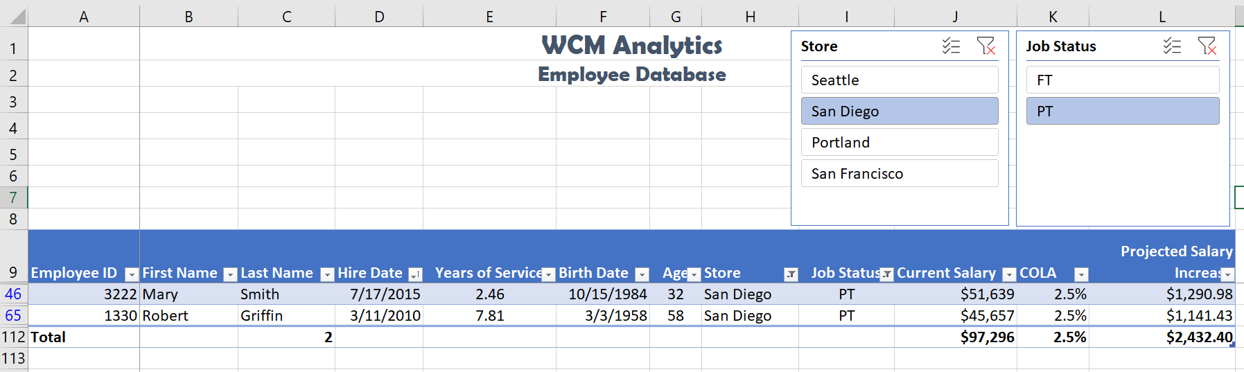
5. From the Store slicer, click the San Diego button. Notice the data filters to only show the data for San Diego.
6. From the Job Status slicer click PT. Notice the data filters to only show the data for PT employees in San Diego.
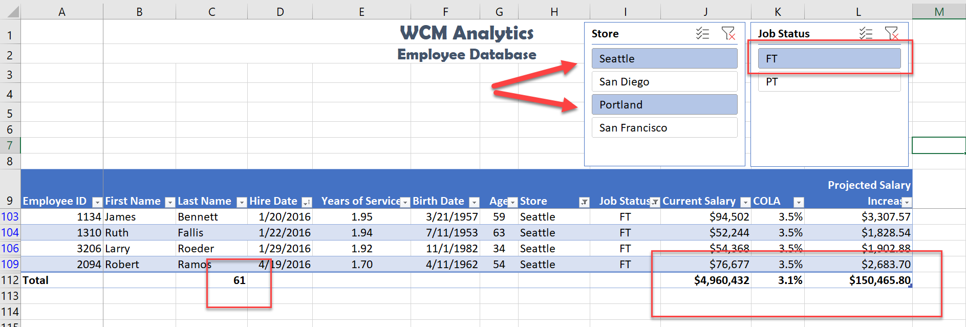
7. Return to the Store slicer and choose Seattle and Portland. Note the non-adjacent selection method is needed. Select Seattle first, then press and hold the Ctrl button on the keyboard, and then select Portland.
![]() Mac Users: hold down the Command key not the Ctrl key before you click on Portland.
Mac Users: hold down the Command key not the Ctrl key before you click on Portland.
8. Change the Job Status slicer selection to FT.
The table results show there are 61 FT employees in Seattle and Portland. The Projected Salary Increase after the COLA adjustment for the Northwest region is $150,465.80.
INSERT TABLE
Often, you’ll have data in a traditional Excel worksheet and want to use the Table features introduced in this chapter. Here’s how to turn a range of data into a Table.
- Select the Over 60 sheet, and click cell A5. This Excel sheet contains a range of data and is not using the Table feature.
- From the Insert tab, choose Table.
- The Create Table dialogue box will appear.
- Make sure “My table has headers” is selected so Excel recognizes the column headings.
- Click OK. Excel turns our advance search data into a table.
- Sort the table in ascending order (A-Z), by Store, and Employee ID, then Last Name. Hint: Click the Data tab, Click the Sort button, add levels for the three fields.
- Save your work.
- A table is made up of a data set that is organized into columns and rows representing fields and records, such as employee information.
- You can create a table by clicking formatting the data set as a table, or using the Insert Table feature.
- Excel offers pre-built table styles, and options to choose from to format a table.
- You can add records (rows) and our fields (columns) to a table. You can then sort to reorganize your data.
- Freezing heading keeps your column headings displayed while you scroll through your table data.
- You can use the filter arrows in the table headings to sort by a single column. When sorting by more than one field, use the Custom Sort option.
- Custom List Sorts can be used when a field needs to be sorted in a special way.
- A slicer is a visual filter button (object) used to filter data in an Excel table. Each unique value in the field is a button.
“5.2 Intermediate Table Skills” by Hallie Puncochar, Portland Community College is licensed under CC BY 4.0
