
Household Budget
Etta and Luca Redding are a couple living in Portland, Oregon. Luca works part time and attends the local community college. Etta works as a marketing manager at a clothing company in North Portland. They are trying to decide if they can afford to move to a better apartment, one that is closer to work and school. They want to use Excel to examine their household budget. They have started their budget spreadsheet, but they need your help with it.
Preparing the Worksheet
- Open the file named PR3 Data and then save it as PR3 Redding.
- Insert two new rows at the top of the worksheet.
- Change the font of entire worksheet to Calibri Light, size 12.
- In cell C2, enter the text Jan (the abbreviation for January).
- Use Autofill to fill in the months Feb through Dec in cells D2:N2. (Hint: Click on cell C2 and drag the fill handle through cells N2)
- In cell O2, enter the text Yearly Total (adjust column width as needed).
- Bold and center align all of the headings in Row 2.
- Type “Redding Family Budget” in A1. Merge & Center A1:O1. Make this text 24 point bold.
- Increase the height of Row 1 to 60px (0.6″). (Hint: Format – Row Height)
- Copy the January values through the other months (February through December) for the following items: (Hint: Use either Copy and Paste or AutoFill)
- Luca’s Income
- Etta’s Income
- Rent
- Renter’s Insurance
- Car Insurance
- Car Payment
- Gas (Car)
- Gym Membership
Calculating Income and Expense totals
- Use the Totals tab in the Quick Analysis tool to add the SUM to Column O. (Hint: Select C3:N24 , click the Quick Analysis Tool button in the bottom-right of the selection, click the Totals tab, then select the SUM column option).
 Mac Users should use the AutoSum tool to calculate the totals in Column O. Since you are using the AutoSum tool, you may not have to delete any formulas in the cells listed in Step 5 above. Also, the Quick Analysis tool will automatically bold the values in Column O. Mac Users should bold cells O3:O45.
 - Delete the SUM functions in the cells for the rows between the categories. (Hint: O6, O12, and O20)
- In C5: N5, use the SUM function to calculate the Total Income for each month.
- Similar to Step 3, use the SUM function to calculate the Total Housing Expenses, Total Essential Expenses, and Total Optional Expenses for each month.
- Format the numerical data in Row 3 as Accounting with no decimal places.
- Format all the total rows as Accounting with no decimal places and with a top border. (Hint: Rows 5, 11, 19, and 24)
- Apply the Comma format with no decimal places in all the other rows. (Hint: Use the Format Painter to make the process quicker)
- In B26, type “Total Expenses”. Apply bold and right-alignment.
- In C26, enter a formula that adds together all of the expense category totals for January. Copy the formula in C26 to the other months and the yearly total (D26:O26). (Hint: the formula for January needs to add C11, C19, and C24).
- Format the data in C26:O26 as Accounting with no decimal places. Bold O26.
- In B28, type “Net Income”. Bold and right-align this text. Also bold C28:028.
- In C28, enter a formula that calculates the difference between Total Income and Total Expenses for January. Copy the formula in C28 to the other months and the yearly total (D28:O28). (Hint: the formula needs to calculate Total Income minus Total Expenses)
- Format the data in B28:O28 and as Accounting with no decimal places. Add a Top and Double Bottom Border to the range of cells.
making a decision
One factor that the Reddings will consider in their decision to move is if their Net Income is positive or negative each month. To help them clearly see this, you will use both data bars and an IF function.
- Add data bars to the Net Income values in C28:O28. The negative values should automatically have a red data bar and the positive values will have a blue data bar. (Hint: Use the Quick Analysis Tool or the Conditional Formatting command on the Home ribbon) Mac Users will need to use the Conditional Formatting tool on the Ribbon.
- In B29, type “Can we afford to move?” and right-align the text.
- Enter an IF statement in C29 that displays the word “No” if the amount in C28 is less than or equal to zero and “Maybe” if the amount is greater than zero. Copy the formula in C29 to the other months (D29:N29). (Hint: the Logical Test needs to be C28<=0)
- Check to see if your IF statement worked correctly in row 29. If the cells say “No” when the data bar in the cell above it is red and “Maybe” when the data bar in the cell above it is blue, your IF statement is correct.
- Change the background (fill) color of A29:O29 to any light shade you prefer.
Finalizing the Worksheet
To increase the readability of the budget worksheet you are going to apply some cell formatting. Take a look at the solution at the end of this section to get an idea of how the worksheet should look when you are finished with this section. 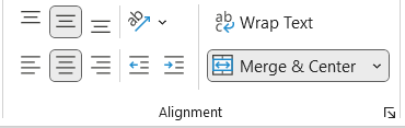
- Merge and Center A3:A5, then change the Vertical Alignment to Middle Align and apply Wrap Text. (Home ribbon – Alignment group)
- Repeat Step 1 for A7:A11, A13:A19, and A21:A24.
- Apply the following borders
- Merged cells – right border (Hint: A3, A7, A13, and A21)
- Total rows – top border (Hint: B5:O5, B11:O11, B19:O19, and B24:O24)
- After each month – right border (Hint: C2:C5, C7:C11, C13:C19, C21:C24, D2:D5, D7:D11, and so on)
- Be sure to apply the right border between the months in rows 26, 28, and 29
- Review the worksheet in Print Preview. Make any changes needed to make the worksheet print on one page with landscape orientation.
- Rename the worksheet to Budget. (Hint: Double-click the Sheet 1 tab, type Budget, and hit Enter)
- Change the color of the worksheet tab to green. (Hint: Right-click the Budget sheet tab, point to Tab Color, and choose a green color) Mac Users should hold down the CTRL key and click the Budget sheet tab
- Check the spelling on all of the worksheets and make any necessary changes. Save the PR3 Redding workbook.
- Compare your work with the answer key below – be sure to click the check marks for details – and then submit the PR3 Redding workbook as directed by your instructor.
Attribution
Adapted from Beginning Excel 2019 and licensed under CC BY.
