
2.2 Introductory Statistical Functions
Learning Objectives
- Use the SUM function to calculate totals.
- Use the COUNT function to count cell locations with numerical values.
- Use the AVERAGE function to calculate the arithmetic mean.
- Use the MAX and MIN functions to find the highest and lowest values in a range of cells.
In addition to formulas, another way to conduct mathematical computations in Excel is through functions. Excel functions apply a mathematical process to a group of cells in a worksheet. For example, the SUM function is used to add the values contained in a range of cells. Functions are more efficient than formulas when you are applying a mathematical process to a group of cells. If you use a formula to add the values in a range of cells, you would have to add each cell location to the formula one at a time. This can be very time-consuming if you have to add the values in a few hundred cell locations. However, when you use a function, you can highlight all the cells that contain values you wish to sum in just one step.
The components of a function are as follows:
=FunctionName(Arguments)
Functions are a type of formula, therefore they start with an equal sign. The next component is the name of the function. A list of commonly used functions is shown in Table 2.4. After the function name comes the arguments for the function, which are always enclosed in parentheses. The arguments are the cell locations and/or values that will be used in the function. The number and type of arguments varies based on the the function being used, although in this section we will only work with a range of cells for the function arguments. Some examples of different functions with their arguments are:
=SUM(B2:B15) – adds the values in B2 through B15
=SQRT(A5) – finds the square root of the value in A5
=COUNTA(A1:A20) – finds the number of cells from A1 through A20 that contain text or a number
Throughout Section 2.2 we will add a variety of mathematical functions to the Personal Budget workbook. In addition to creating functions, this section also reviews percent of total calculations and the use of absolute references.
Table 2.4 Commonly Used Functions
| Function | Output |
| ABS | The absolute value of a number |
| AVERAGE | The average or arithmetic mean for a group of numbers |
| COUNT | The number of cell locations in a range that contain a numeric value |
| COUNTA | The number of cell locations in a range that contain text or a numeric value |
| MAX | The highest numeric value in a group of numbers |
| MEDIAN | The middle number in a group of numbers (half the numbers in the group are higher than the median and half the numbers in the group are lower than the median) |
| MIN | The lowest numeric value in a group of numbers |
| MODE | The number that appears most frequently in a group of numbers |
| PRODUCT | The result of multiplying all the values in a range of cell locations |
| SQRT | The positive square root of a number |
| SUM | The total of all numeric values in a group |
It is important to note that there are several methods for adding a function to a worksheet, and we will explore each of them throughout this section.
- Typing the function directly into a cell
- Selecting from the function list
- Using the Function Library on the ribbon
- Using the Insert Function button
The SUM Function
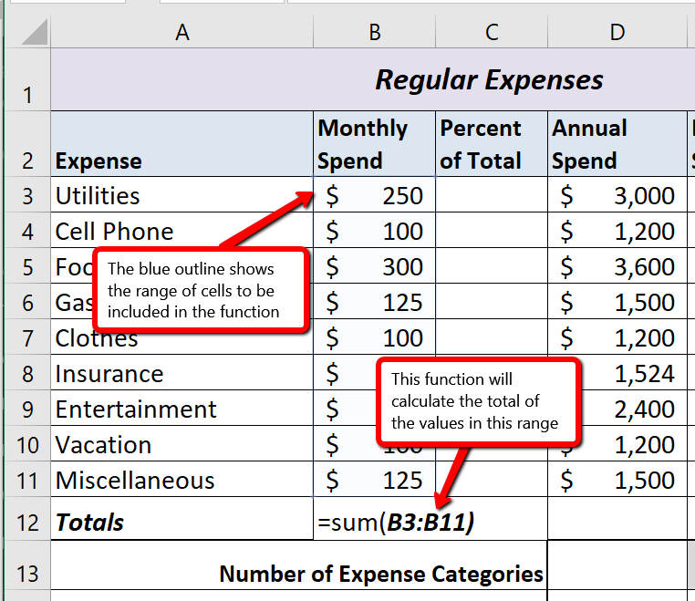
The SUM function is used when you need to calculate totals for a range of cells or a group of selected cells on a worksheet. With regard to the Budget Detail worksheet, we will use the SUM function to calculate the totals in row 12, starting with the Monthly Spend total in B12. The following illustrates how a function can be added to a worksheet by typing it into a cell location:
=SUM(B3:B11) calculates the total of the values
in cells B3 through B11
- Switch to the Budget Detail worksheet if needed.
- Click cell B12.
- Type an equal sign =.
- Type the function name SUM.
- Type an open parenthesis (.
- Click cell B3 and drag down to cell B11. This places the range B3:B11 into the function.
- Type a closing parenthesis ).
- Press the ENTER key. The function calculates the total for the Monthly Spend column, which is $1,427.
Figure 2.11 shows the appearance of the SUM function added to the Budget Detail worksheet before pressing the ENTER key.
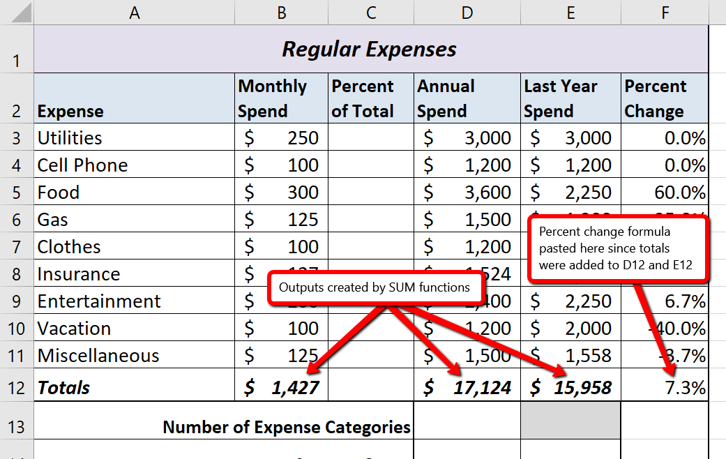
As shown in Figure 2.11, the SUM function was added to cell B12. However, this function is also needed to calculate the totals in the Annual Spend and Last Year Spend columns. The function can be copied and pasted into these cell locations because of relative referencing. Relative referencing serves the same purpose for functions as it does for formulas. To complete the Totals in row 12, we need to copy and paste the SUM function into D12 and E12. Since we will then have totals in D12 and E12, we can paste the percent change formula into F12.
- Click cell B12 in the Budget Detail worksheet.
- Click the Copy button in the Home tab of the Ribbon.
- Highlight cells D12 and E12.
- Click the Paste button in the Home tab of the Ribbon. This pastes the SUM function into cells D12 and E12 and calculates the totals for these columns.
- Click cell F11.
- Click the Copy button in the Home tab of the Ribbon.
- Click cell F12, then click the Paste button in the Home tab of the Ribbon.
Figure 2.12 shows the output of the SUM function that was added to cells B12, D12, and E12. In addition, the percent change formula was copied and pasted into cell F12. Notice that this version of the budget is planning an increase in spending compared to last year.
Cell Ranges in Functions
When you intend to use a function on a range of cells in a worksheet, make sure there are two cell locations separated by a colon and not a comma. If you enter two cell locations separated by a comma, the function will calculate only the two cell locations listed instead of an entire range of cells. For example, the SUM function shown in Figure 2.13 will add only the values in cells C3 and C11, not the range C3:C11.
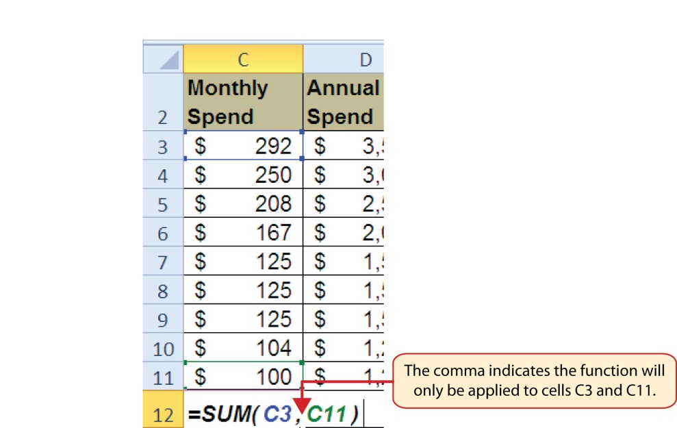
Figure 2.13 SUM Function Adding Two Cell Locations
The COUNT Function
The next function that we will add to the Budget Detail worksheet is the COUNT function. The COUNT function is used to determine how many cells in a range contain a numeric entry. The COUNT function will not work for counting text or other non-numeric entries. If you want to count text instead of, or in addition to, numeric entries you use the COUNTA function. For the Budget Detail worksheet, we will use the COUNT function to count the number of items that are planned in the Annual Spend column (Column D). The following explains how the COUNT function is added to the worksheet by selecting from the function list:
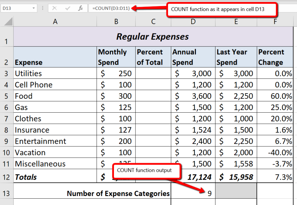
=COUNT(D3:D11) will count how many cells contain numeric values in the range D3 through D11
- Click cell D13.
- Type an equal sign =.
- Type the letter C (to start spelling the name of the function).
- Click the down arrow on the scroll bar of the function list (see Figure 2.14) and find the word COUNT.
 Mac Users can scroll down with touchpad or mouse to find COUNT
 - Double click the word COUNT from the function list.
Mac Users should single click the word “COUNT” do not double-click - Highlight the range D3:D11.
- You can type a closing parenthesis ) and then press the ENTER key, or simply press the ENTER key and Excel will close the function for you. The function produces an output of 9 since there are 9 items planned on the worksheet.
Figure 2.14 shows the function list box that appears after completing steps 2 and 3 for the COUNT function. The function list provides an alternative method for adding a function to a worksheet.
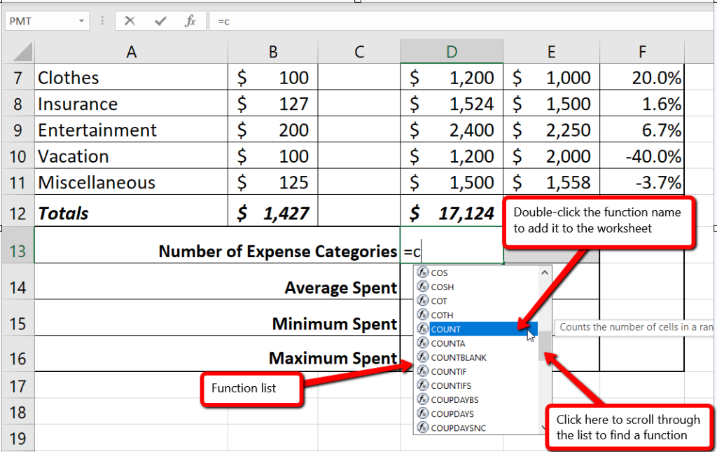
Figure 2.15 shows the output of the COUNT function after pressing the ENTER key. The function counts the number of cells in the range D3:D11 that contain a numeric value. The result of 9 indicates that there are 9 categories planned for this budget.
The AVERAGE Function
The next function we will add to the Budget Detail worksheet is the AVERAGE function. This function is used to calculate the arithmetic mean (average) for a group of numbers. For the Budget Detail worksheet, we will use the function to calculate the average of the values in the Annual Spend column. We will add this to the worksheet by using the Function Library on the Formulas ribbon. The following steps explain how this is accomplished:
=AVERAGE(D3:D11) will calculate the average of the values in the range D3 through D11
- Click cell D14 in the Budget Detail worksheet.
- Click the Formulas tab on the Ribbon.
- Click the More Functions button in the Function Library group of commands.
- Place the mouse pointer over the Statistical option from the drop-down list of options.
- Click the AVERAGE function name from the list of functions that appear in the menu (see Figure 2.16). This opens the Function Arguments dialog box.
- Click the Collapse Dialog button in the Function Arguments dialog box (see Figure 2.17).
For Mac Users, the Collapse Dialog button may not collapse. Just continue with Step 7 and press Enter after selecting the range. - Highlight the range D3:D11.
- Click the Expand Dialog button in the Function Arguments dialog box (see Figure 2.18). You can also press the ENTER key to get the same result.
- Click the OK button on the Function Arguments dialog box. This adds the AVERAGE function to the worksheet.
Mac Users should click the DONE button
Figure 2.16 illustrates how a function is selected from the Function Library in the Formulas tab of the Ribbon.
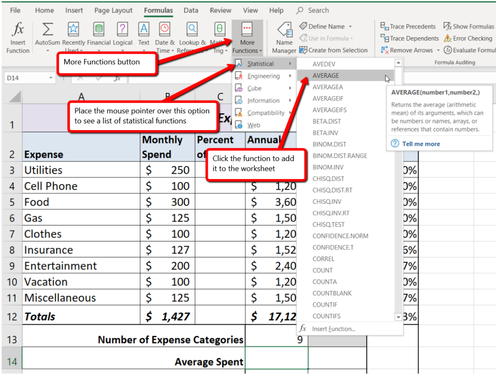
Figure 2.17 shows the Function Arguments dialog box. This appears after a function is selected from the Function Library. The Collapse Dialog button is used to hide the dialog box so a range of cells can be highlighted on the worksheet and then added to the function.
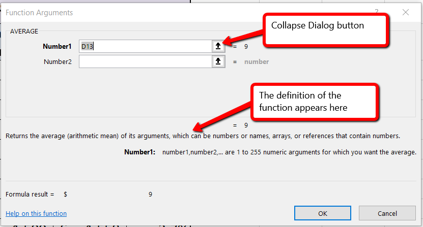
Figure 2.18 shows how a range of cells can be selected from the Function Arguments dialog box once it has been collapsed.
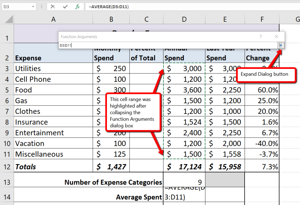
Figure 2.19 shows the Function Arguments dialog box after the cell range is defined for the AVERAGE function. The dialog box shows the result of the function before it is added to the cell location. This allows you to assess the function output to determine whether it makes sense before adding it to the worksheet.
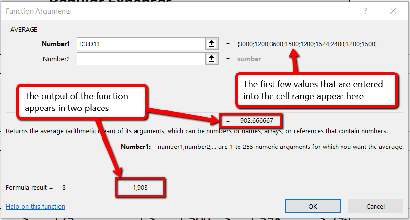
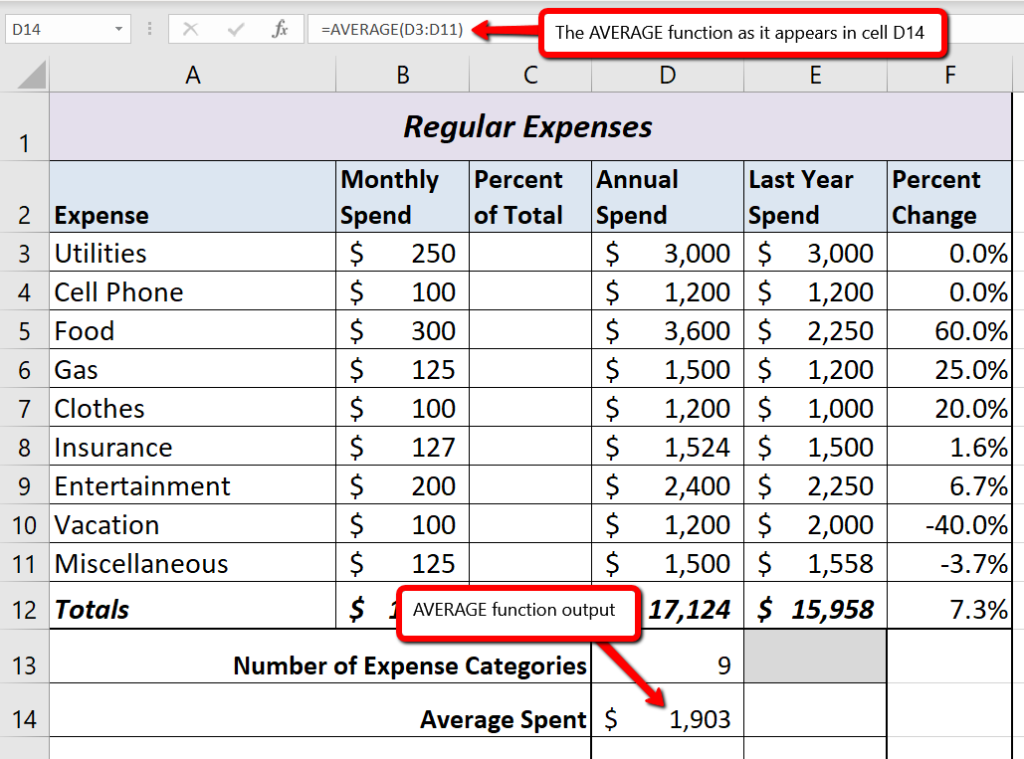
Figure 2.20 shows the completed AVERAGE function in the Budget Detail worksheet. The output of the function shows that on average we expect to spend $1,903 for each of the categories listed in Column A of the budget. This average spend calculation per category can be used as an indicator to determine which categories are costing more or less than the average budgeted spend dollars.
The MAX and MIN Functions
Data file: Continue with CH2 Personal Budget.
The final two statistical functions that we will add to the Budget Detail worksheet are the MAX and MIN functions. These functions identify the highest and lowest values in a range of cells. The following steps explain how to add these functions to the Budget Detail worksheet using the Insert Function button:
=MAX(D3:D11) will find the largest value in the range of cells D3 through D11
=MIN(D3:D11) will find the smallest value in the range of cells D3 through D11
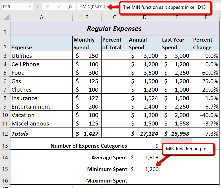
- Click cell D15 in the Budget Detail worksheet.
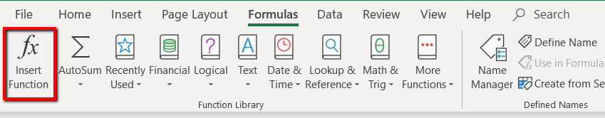
- Click the Insert Function button on the Formulas ribbon. (see Figure 2.21)
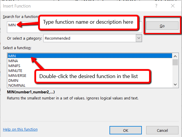
- This brings up the Insert Function dialog box. Type the word MIN in the search box and then click the Go button. (see Figure 2.22)
- Double-click MIN in the list. This opens the Function Arguments dialog box.
- Click the Collapse Dialog button in the Function Arguments dialog box.
- Highlight the range D3:D11.
- Click the Expand Dialog button in the Function Arguments dialog box.
- Click the OK button on the Function Arguments dialog box. This adds the MIN function to the worksheet. (see Figure 2.23)
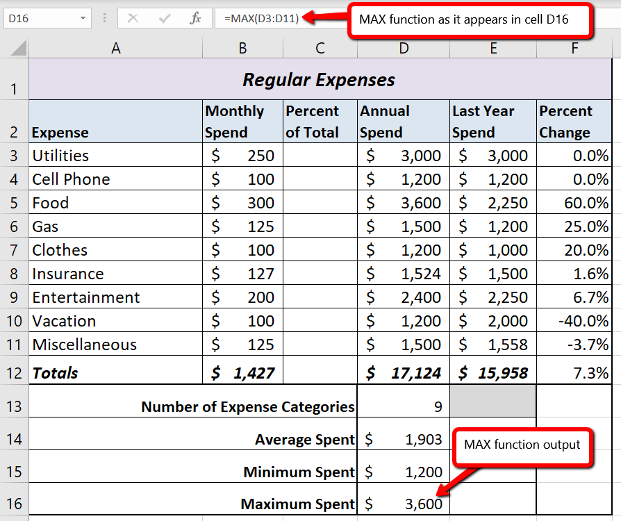
- Click cell D16.
- Repeat steps 2-8 (using MAX instead of MIN) to add the MAX function to the worksheet. (see Figure 2.24)
Skill Refresher
Typing a function or selecting from the function list
- Type an equal sign =.
- Type the function name followed by an open parenthesis ( or double click the function name from the function list.
- Highlight the range of cells to use or click individual cell locations followed by commas.
- Type a closing parenthesis ) and press the ENTER key or press the ENTER key to close the function.
Inserting a function using the ribbon
- On the Formulas ribbon, select the correct category in the Function Library. Click the desired function in the list.
- In the Function Dialog box, click the Collapse Dialog button and highlight the range of cells to use.
- Click the Expand Dialog button and then click the OK button in the Function Arguments dialog box.
Inserting (and searching for) a function using the Insert Function button
- On the Formulas ribbon, click the Insert Function button and search for the function to use. Double-click on the desired function in the list.
- In the Function Dialog box, click the Collapse Dialog button and highlight the range of cells to use.
- Click the Expand Dialog button and then click the OK button in the Function Arguments dialog box.
Key Takeaways
- Statistical functions are used when a mathematical process is required for a range of cells, such as summing the values in several cell locations. For these computations, functions are preferable to formulas because adding many cell locations one at a time to a formula can be very time-consuming.
- Statistical functions can be created using cell ranges or selected cell locations separated by commas. Make sure you use a cell range (two cell locations separated by a colon) when applying a statistical function to a contiguous range of cells.
- To prevent Excel from changing the cell references in a formula or function when they are pasted to a new cell location, you must use an absolute reference. You can do this by placing a dollar sign ($) in front of the column letter and row number of a cell reference.
- The #DIV/0 error appears if you create a formula that attempts to divide a constant or the value in a cell reference by zero.
Attribution
Adapted from Beginning Excel 2019 and licensed under CC BY.
