midasCoffee Company

Ruth Kobran owns a coffee supply company named MidasCoffee. She needs some help writing the formulas for the order form she uses to invoice customers. You will to enter VLOOKUP functions to to fill in the description and unit price on the order form. Additionally will need to write the formulas for all of the calculations on the form. Some of the more complex parts are determining if the customer will get a discount (based on the customer status) as well as the shipping charge (orders over $199 get free shipping). You will use IF functions for both of those calculations. Then you will analyze some sales data for the six MidasCoffee company locations in the Portland area by creating two PivotTables that will answer two different questions about the sales data.

Prepare the Worksheet

1. Open the SC3 Data workbook and save the workbook as SC3 MidasCoffee.
2. Enter the following order information:
   Order #: 56894
   Order Date: use a function that displays the current date
3. Enter the following Billing Information:
   Samantha Raitt
   4270 SW Cooper Ln
   Portland, OR 97225
   503-674-1632
   samantha.raitt@zmail.com
4. For the Shipping Information, create formulas using cell references to display the corresponding information from the Billing Information section. For example, the Customer cell will display the name of the customer in cell C11.
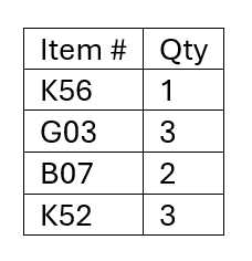
5. In the range B19:B22 and D19:D22 enter the following item numbers and Quantities:

Create Formulas and Functions

1. In cell C19 enter a VLOOKUP function that will return the description of the item number in cell B19. The Lookup Table in on the Lookup Table sheet.
2. Copy/fill this formula down through row 25. Excel will return the #N/A error message for any rows that do not have an item # entered.
3. To fix the error messages, we’ll add the IFERROR function to the VLOOKUP function. The IFERROR function will insert what we tell it to in the cell if an error message appears.
   1. Click in cell C19 to make it active.
   2. In the formula bar, click right after the equal sign in the VLOOKUP function.
   3. Key in the letters if to bring up the IFERROR function and double click on it to select it.
   4. Move to the very end of the function, after the closing parenthesis.
   5. Type a comma, then two quotation marks (“”). The two quotation marks mean to insert a blank space.
   6. Type the closing parenthesis mark and push the Enter key on your keyboard.
      1. The formula will look like this: =IFERROR(VLOOKUP(Lookup value, Table array, Col index num, FALSE),””)
   7. Refill the function down through row 25. This should eliminate the error messages. If not, repeat the above steps.
4. In cell E19 enter another VLOOKUP function to retrieve the Unit Price from the Lookup Table.
5. Edit the VLOOKUP function in cell E19 to add the IFERROR function that same as you did for cell C19
6. Fill the function down through row 25.
7. In cell F19, enter an IF function that tests whether the order quantity in cell D19 is greater than 0 (zero). lf it is, return the value of the Qty (in D19) multiplied by the Unit Price (in E19); otherwise, return no text by entering “”. Hint: You will need to use a formula for the Value if True argument.
8. Copy/fill this formula into the other cells in the range F19:F25. Hint: be sure to copy the formula to all of the Item Total cells, even if it is a blank row. You want the worksheet to be prepared for orders with more items in the future.
9. In cell F26, calculate the sum of all of the Item Total cells.
10. In cell F27, use an IF function to calculate the discount amount for this order based on the customer’s status (which is found in F16). If the customer’s status is Preferred, the discount amount will be the Order Subtotal times the discount percentage found in cell B29; otherwise the discount amount will be 0 (zero). Hint: You will need to use a formula for the Value if True argument. 
11. Use the drop-down list to change the customer’s Status in cell F16 to Regular. Make sure you do not end up with an error message in cell F27. If you get an error message, check the IF function and make the changes needed.
12. Change the customer’s Status back to Preferred. Try different values to make sure your IF functions work for both True and False results.
13. Calculate the Discounted Total for this order in cell F28. Hint: Use a simple subtraction formula.
14. In cell F29, use an IF function to display the correct Shipping Charge, based on the amount of the Discounted Total. If the Discounted Total is greater than or equal to the Free Shipping Minimum found in cell B28, the Shipping Charge is 0 (zero); otherwise, the Shipping Charge is 5% of the Discounted Total. Hint: You will need to use a formula for the Value if False to calculate what 5% of the Discounted Total will be.
15. Calculate the Invoice Total in cell F31. Hint: This will be the total of the Discounted Total and the Shipping Charge. The Invoice Total should be $107.64. If you do not get this number, go back and find your error and correct it.

Create PivotTables

1. Change to the Coffee Sales sheet. On this sheet is sales data for the four Midas Coffee locations in the Portland area, showing the date, coffee type, quantity sold, total sales, and location.
2. Look at the data and determine what questions you could ask about this data. One question could be, “Which coffee type had the highest sales?”
3. Let’s build a PivotTable to answer this question. Begin by inserting a blank, new PivotTable on the Coffee Sales sheet in cell H2.
4. What fields would you need to show which coffee type had the highest sales–select the Coffee Type and Total Sales ($) fields in the PivotTable Fields panel.
5. Format the PivotTable appropriately–adjust column widths and labels, format numbers (Remember the best way to format numbers in a PivotTable?), and give the PivotTable a name in the PivotTable Name box on the PivotTable Analyze tab.
6. By viewing the PivotTable data, determine the coffee type with the highest sales. In cell K2 of the Coffee Sales sheet, type in your answer.
7. Several rows underneath the PivotTable, type in a second question you could ask about this data. There are several possibilities, so there is not just one correct answer. Format the question in bold text with a larger font.
8. Three rows under the second question, insert a blank, new PivotTable and add the appropriate fields to answer your second question.
9. Format this PivotTable appropriately.
10. In the row underneath you second question, type in the answer to your question based on the information from the second PivotTable.

Finalizing the Worksheet

1. Take a critical look at your worksheets to ensure that all of the number and cell formatting is professional.
2. Review the worksheets in Print Preview. Make any changes needed to make the worksheets print on one page.
3. Check the spelling on all of the worksheets and make any necessary changes. Save the SC3 MidasCoffee workbook.
4. Submit the SC3 Midas Coffee workbook as directed by your instructor.

Attribution

Adapted from Beginning Excel 2019 and licensed under CC BY.