
2.3 Copy and Paste Formulas, and Absolute Cell References
Learning Objectives
- Learn how to copy and paste formulas without formats applied to a cell location.
- Use absolute references to calculate percent of totals.
Copy and Paste Formulas (Pasting without Formats)
As shown in Figure 2.24, the COUNT, AVERAGE, MIN, and MAX functions are summarizing the data in the Annual Spend column. You will also notice that there is space to copy and paste these functions under the Last Year Spend column. This allows us to compare what we spent last year and what we are planning to spend this year. Normally, we would simply copy and paste these functions into the range E14:E16. However, you may have noticed the thicker style border that was used around the perimeter of the range D13:E16. If we used the regular Paste command, the thick line on the right side of the range D13:E16 would be replaced with a single line. Therefore, we are going to use one of the Paste Special commands to paste only the functions without any of the formatting treatments. This is accomplished through the following steps:
- Highlight the range D14:D16 in the Budget Detail worksheet.
- Click the Copy button in the Home tab of the Ribbon.
- Click cell E14.
- Click the down arrow below the Paste button in the Home tab of the Ribbon.
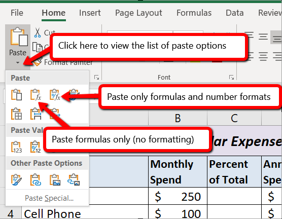
- Click the Formulas option from the drop-down list of buttons (see Figure 2.25).
Figure 2.25 shows the list of buttons that appear when you click the down arrow below the Paste button in the Home tab of the Ribbon. One thing to note about these options is that you can preview them before you make a selection by dragging the mouse pointer over the options. When the mouse pointer is placed over the Formulas button, you can see how the functions will appear before making a selection. Notice that the thick line border does not change when this option is previewed. That is why this selection is made instead of the regular Paste option.
Skill Refresher
Paste Formulas without formatting
- Click a cell location containing a formula or function.
- Click the Copy button in the Home tab of the Ribbon.
- Click the cell location or cell range where the formula or function will be pasted.
- Click the down arrow below the Paste button in the Home tab of the Ribbon.
- Click the Formulas button under the Paste group of buttons.
Absolute References (Calculating Percent of Totals)
To further analyze your budget, you want to see what percentage of your total monthly spending is spent in each category. Since totals were added to row 12 of the Budget Detail worksheet, a percent of total calculation can be added to Column C beginning in cell C3. The percent of total calculation shows the percentage for each value in the Monthly Spend column with respect to the total in cell B12. However, after the formula is created, it will be necessary to turn off Excel’s relative referencing feature before copying and pasting the formula to the rest of the cell locations in the column. Turning off Excel’s relative referencing feature is accomplished through an absolute reference.
First we will create the formula, which needs needs to divide the amount in B3 by the total monthly spend in B12. This formula is =B3/B12
- Click cell C3 in the Budget Detail worksheet.
- Type an equal sign =.
- Click cell B3.
- Type a forward slash /.
- Click cell B12.
- Press the ENTER key. You will see that Utilities represent about 17.5% of the Monthly Spend budget (see Figure 2.26).
- Figure 2.26 shows the completed formula that is calculating the percentage that Utilities represents to the total Monthly Spend for the budget (see cell C3). Normally, we would copy this formula and paste it into the range C4:C11. However, because of relative referencing, both cell references will increase by one row as the formula is pasted into the cells below C3. This is fine for the first cell reference in the formula (C3) but not for the second cell reference (C12).Figure 2.26 illustrates what happens if we paste the formula into the range C4:C12 in its current state. Notice that Excel produces the #DIV/0 error code. This means that Excel is trying to divide a number by zero, which is impossible. Looking at the formula in cell C4, you see that the first cell reference was changed from B3 to B4. This is fine because we now want to divide the Monthly Spend for Cell Phone (cell B4) by the total Monthly Spend in cell B12. However, Excel has also changed the B12 cell reference to B13. Because cell location B13 does not contain a number, the formula produces the #DIV/0 error code.
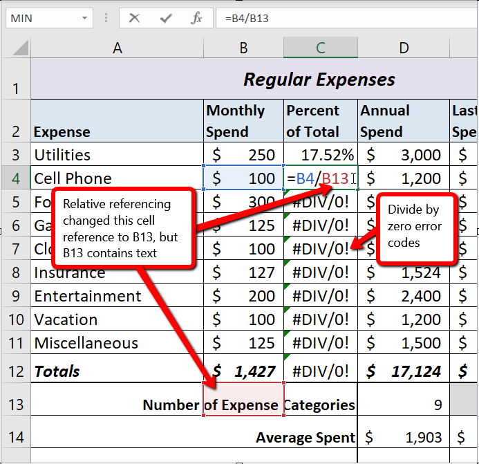
Figure 2.26 #DIV/0 Error from Relative Referencing To eliminate the divide-by-zero error shown in Figure 2.26 we must add an absolute reference to cell B12 in the formula. An absolute reference prevents relative referencing from changing a cell reference in a formula. This is also referred to as locking a cell. No matter where you copy a formula with an absolute reference, it will always refer back to the locked cell. An absolute reference is indicated by a $ sign in front of both the column letter and the row number. For example, $A$15 is an absolute reference to cell A15.
$B$12 is an example of
an absolute referenceWe are going to modify the existing formula in C3 to make the reference to cell B12 an absolute reference. The revised formula will be =B3/$B$12. The following explains how this is accomplished:
- Double click cell C3.
- Place the mouse pointer in front of B12 and click. The blinking cursor should be in front of the B in the cell reference B12.
- Press the F4 key. You will see a dollar sign ($) added in front of the column letter B and the row number 12. You can also type the dollar signs in front of the column letter and row number if you prefer. The formula should appear as =B3/$B$12. The F4 key is a cool shortcut for adding the dollar signs.
 Mac Users: If the F4 key does not insert the $ symbols, check the keyboard settings: click black Apple icon
  at top left of the screen, choose “System Preferences”, click the Keyboard icon, make sure the checkbox is checked for the item that says: “Use F1, F2, etc. as standard function keys”.
 - Press the ENTER key.
- Click cell C3.
- Use the AutoFill Handle or Copy and Paste to copy the formula from C3 to the range C4:C11.
Figure 2.27 shows the percent of total formula with an absolute reference added to B12. Notice that in cell C4, the cell reference remains B12 instead of changing to B13. Also, you will see that the percentages are being calculated in the rest of the cells in the column, and the divide-by-zero error is now eliminated.
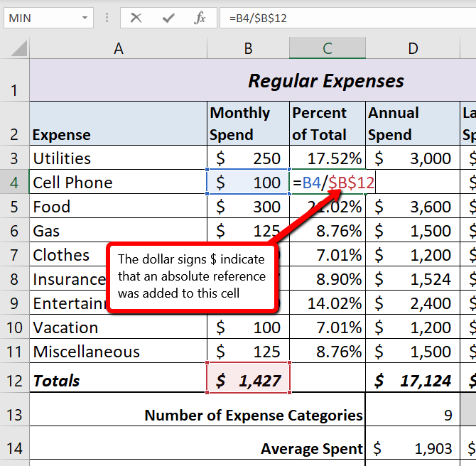
Figure 2.27 Adding an Absolute Reference to a Cell Reference in a Formula Skill Refresher
Absolute References
- Click in front of the column letter of a cell reference in a formula or function that you do not want altered when the formula or function is pasted into a new cell location.
- Press the F4 key or type a dollar sign $ in front of the column letter and row number of the cell reference.
Key Takeaways
Type your key takeaways here.
- To prevent Excel from changing the cell references in a formula or function when they are pasted to a new cell location, you must use an absolute reference. You can do this by placing a dollar sign ($) in front of the column letter and row number of a cell reference.
- The #DIV/0 error appears if you create a formula that attempts to divide a constant or the value in a cell reference by zero.
- The Paste Formulas option is used when you need to paste formulas without any formatting treatments into cell locations that have already been formatted.
Attribution
Adapted from Beginning Excel 2019 and licensed under CC BY.
