Sorting Data (Multiple Levels)

The Budget Detail worksheet shown in Figure 2.28 is now producing several mathematical outputs through formulas and functions. The outputs allow you to analyze the details and identify trends as to how money is being budgeted and spent. Before we draw some conclusions from this worksheet, we will sort the data based on the Percent of Total column. Sorting is a powerful tool that enables you to analyze key trends in any data set. Sorting will be covered thoroughly in a later chapter, but will be briefly introduced here.

For the purposes of the Budget Detail worksheet, we want to set multiple levels for the sort order.  We are going to sort first by the Percent of Total, and then by the Last Year Spend amount.  Excel will first sort the items by the Percent of Total, and any items with the same Percent of Total will then be sorted by Last Year Spend. This is accomplished through the following steps:

1. Highlight the range A2:F11.
2. Click the Data tab in the Ribbon.
3. Click the Sort button in the Sort & Filter group of commands. This opens the Sort dialog box, as shown in Figure 2.28.
4. Click the down arrow next to the “Sort by” box.
5. Click the Percent of Total option from the drop-down list.
6. Click the down arrow next to the sort Order box.
7. Click the Largest to Smallest option.
8. Click the Add Level button. This allows you to set a second level for any duplicate values in the Percent of Total column.
    the + symbol at bottom left corner is the “Add Level” button for Excel for Mac
9. Click the down arrow next to the “Then by” box.
10. Select the Last Year Spend option. Leave the Sort Order as Smallest to Largest
11. Click the OK button at the bottom of the Sort dialog box.
12. Save the CH2 Personal Budget file.

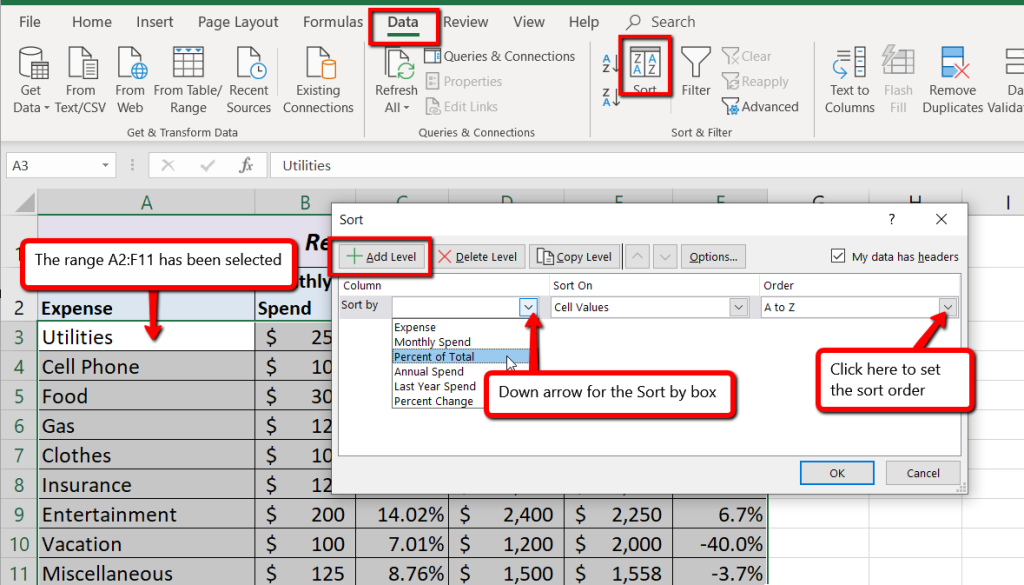
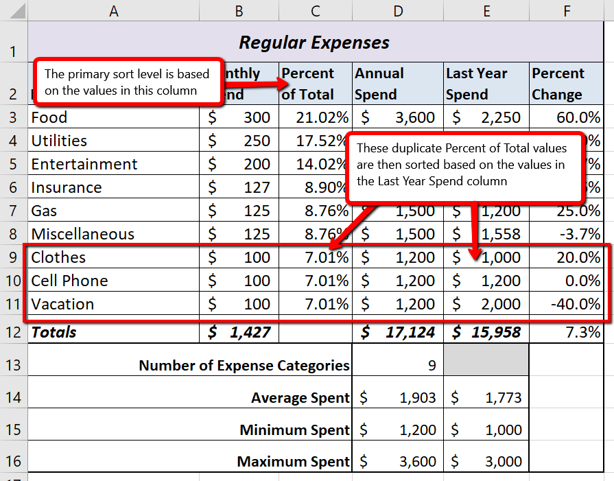
Figure 2.29 shows the Budget Detail worksheet after it has been sorted. Notice that there are three identical values in the Percent of Total column. This is why a second sort level had to be created for this worksheet. The second sort level arranges the values of 7.01% based on the values in the Last Year Spend column in ascending order. Excel gives you the option to set as many sort levels as necessary for the data contained in a worksheet.

Filtering Data

Sometimes we are working with a large data set and we want to narrow down the rows of data to focus on a particular subset. To do this, we can filter the data in a data range to display only the information we want to focus on at the moment. You can filter by various criteria. If you were working with cities and states, you can use a text filter to only show the state of Oregon. When working with numbers, you can use chose from different number filters such as greater than, equal to, less than, etc.

In our Budget Detail worksheet, we will filter the data to only show those expenses that had a percent change greater than 15%. First we will turn on the AutoFilter arrows for each column in our data.

1. On the Budget Detail sheet, click anywhere in the range A2:F11.
2. Click the Data tab in the Ribbon.
3. In the Sort & Filter group, click on the large Filter icon. When you click on this command, Excel adds AutoFilters to each column. These are the small dropdown arrows next to the column headings. When you click on one of these AutoFilters you will see different options for filtering the data in that column. If it’s a text column, you will have a text filter and if it’s a number column, you’ll see number filters. Figure 2.30 shows the Budget Detail worksheet with the AutoFilter buttons.
   

   

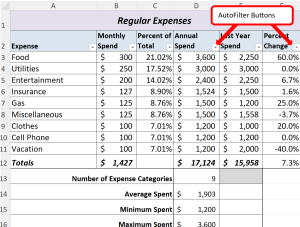
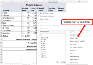
4. Click on the AutoFilter button for the Percent Change column. Figure 2.31. First, you’ll see sort options at the top of the list, so this is another way to sort data. Towards the bottom there is a list of all of the data points in this column. We can use this list to filter down to show only the data points we want to display. However, using the Number Filters option is more efficient.
   

   

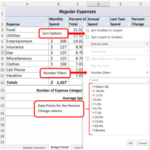
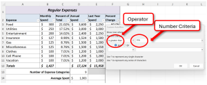
5. Point to Number Filters, then, in the next menu that appears, click on Greater Than… (See Figure 2.32) This opens the Custom Autofilter dialog box, as shown in Figure 2.33. Since we selected Greater Than, that is the option displaying in the first box and we will not change this. Key in 15% or .15 in the next box because we want to only display expense items that have a percent change greater than 15%. Click OK

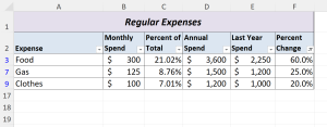
This filters the data to only show items with a percent change greater than 15%. Three expense items display: Food, Gas, and Clothes.  See Figure 2.34. Our other expense items are not deleted, they are just hidden.

6. To remove the filter and display all of the items again, click on the large Filter icon in the Sort & Filter group in the Data tab on the ribbon, this also removes the AutoFilter buttons from the data. Alternatively, you can click on the AutoFilter button next to the column label and click on “Clear Filter from Percent Change,” this will not remove the AutoFilter buttons if you want to filter by another field.

7. Save the CH2 Personal Budget file.