Linking Worksheets (Creating a Summary Worksheet)

So far we have used cell references in formulas and functions, which allow Excel to produce new outputs when the values in the cell references are changed. Cell references can also be used to display values or the outputs of formulas and functions in cell locations on other worksheets. This is how we will complete the Budget Summary worksheet using values from both the Budget Detail and Loan Payments worksheets.

Outputs from the formulas and functions that were entered into the Budget Detail will be displayed on the Budget Summary worksheet through the use of cell references.

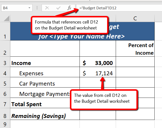
1. Switch to the Budget Summary worksheet and select cell B4. This cell needs to reference the Total Annual Spend (D12) from the Budget Detail worksheet.
2. Type an =
3. Click the Budget Detail worksheet tab.
4. Click cell D12.
5. Press the ENTER key on your keyboard.
6. The formula bar will display the formula =’Budget Detail’!D12 and the cell will display $17,124. (see Figure 2.43)

Figure 2.43 shows how the cell reference appears in the Budget Summary worksheet. Notice that the cell reference D12 is preceded by the Budget Detail worksheet name enclosed in apostrophes followed by an exclamation point (‘Budget Detail’!) This indicates that the value displayed in the cell is referencing a cell location in the Budget Detail worksheet.

We will use a similar process to enter in the annual car payments and mortgage payments from the Loan Payments worksheet.  The payments on the Loan Payments worksheet are monthly payments though, so we will need to multiply each one by 12 to get the annual amount to display in the Budget Summary worksheet.

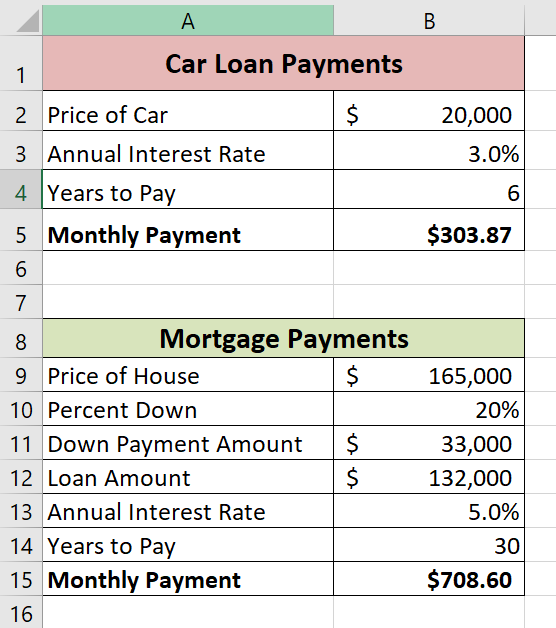
1. Click on cell B5. This cell needs to contain a formula that references the monthly car payment cell (B5) on the Loan Payments worksheet and multiplies by 12.
2. Type an =
3. Click the Loan Payments worksheet tab.
4. Click cell B5 on the Loan Payments worksheet.
5. The formula bar will display the formula =’Loan Payments’!B5 
6. Type an asterisk * for multiplication.
7. Type the number 12. The formula in the formula bar should read: =’Loan Payments’!B5*12
8. Press the ENTER key on your keyboard.
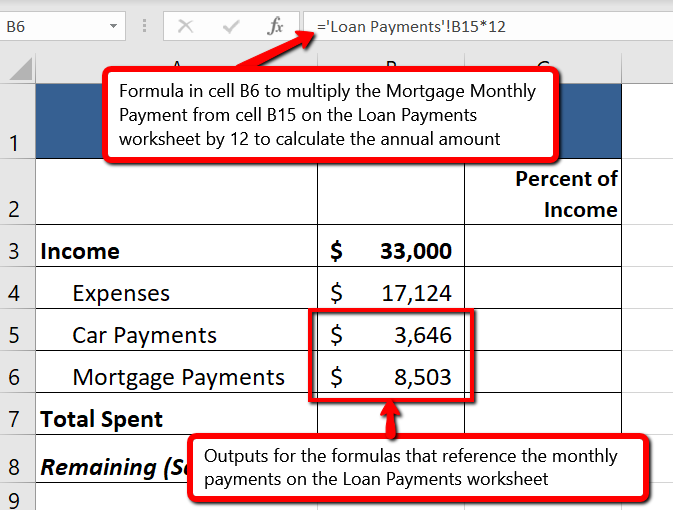
9. Click on cell B6. This cell needs to contain a formula that references the monthly mortgage payment cell (B15) on the Loan Payments worksheet and multiplies by 12.
10. Type an =
11. Click the Loan Payments worksheet tab.
12. Click cell B15 on the Loan Payments worksheet.
13. The formula bar will display the formula =’Loan Payments’!B15 
14. Type an asterisk * for multiplication.
15. Type the number 12. The formula in the formula bar should read: =’Loan Payments’!B15*12
16. Press the ENTER key on your keyboard.

Figure 2.44 shows the results of creating formulas that reference cell locations in the Loan Payments worksheet.

We can now add other formulas and functions to the Budget Summary worksheet that can calculate the difference between the total spend dollars vs. the total net income in cell B3. The following steps explain how this is accomplished:

1. Click cell B7 in the Budget Summary worksheet.
2. Type an equal sign =.
3. Type the function name SUM followed by an open parenthesis (.
4. Highlight the range B4:B6.
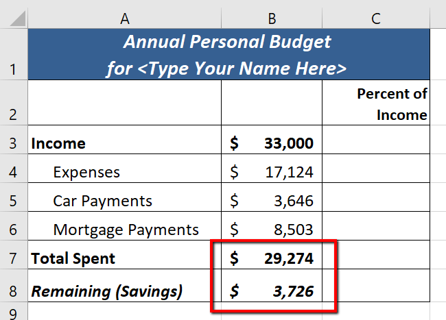
5. Type a closing parenthesis ) and press the ENTER key on your keyboard or simply press the ENTER key to close the function. The total for all annual expenses now appears on the worksheet.
6. Click cell B8 on the Budget Summary worksheet. You will enter a formula to calculate Remaining (Savings) amount in this cell.
7. Type an equal sign =.
8. Click cell B3.
9. Type a minus sign − and then click cell B7.
10. Press the ENTER key on your keyboard. This formula produces a positive number, indicating our income is greater than our total expenses.

Figure 2.45 shows the results of the formulas that were added to the Budget Summary worksheet. Overall, having your income exceed your total expenses is a good thing because it allows you to save money for future spending needs or unexpected events.

We can now add a few formulas that calculate both the spending rate and the savings rate as a percentage of net income. These formulas require the use of absolute references, which we covered earlier in this chapter. The following steps explain how to add these formulas:

1. Click cell C7 in the Budget Summary worksheet.
2. Type an equal sign =.
3. Click cell B7.
4. Type a forward slash / for division and then click B3.
5. Press the F4 key on your keyboard. This adds an absolute reference to cell B3.
6. Press the ENTER key. The result of the formula shows that total expenses consume  89% of our net income.
7. Click cell C7.
8. Place the mouse pointer over the Auto Fill Handle.
9. When the mouse pointer turns to a black plus sign, left click and drag down to cell C8. This copies and pastes the formula into cell C8.
10. Compare your worksheets with Figures 2.41a-c below.  Make any necessary changes before moving on to the next section.
11. Save the CH2 Personal Budget file.

Figure 2.46a shows the completed Budget Summary worksheet

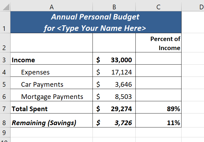
Figure 2.46b shows the completed Budget Detail worksheet

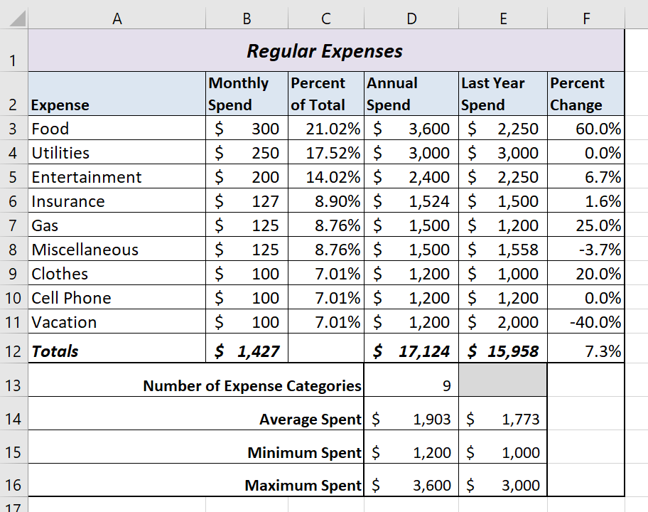
Figure 2.46c shows the completed Loan Payments worksheet

Attribution

Adapted from Beginning Excel 2019 and licensed under CC BY.