
3.4 Introduction to PivotTables
PivotTables
While conditional formatting, which you learned about in the previous section, provides one way to emphasize key points in your data, another way to analyze data is by using PivotTables. PivotTables are a powerful tool that can help make your worksheets more manageable by summarizing your data and allowing you to manipulate it in different ways. PivotTables are inserted directly from the contents of a dataset, linking to the data but using a summary table format while the original dataset remains unchanged. We will do a brief introduction to PivotTables here so you become familiar with this widely used Excel tool.
First, click the link below to view a video on PivotTables:
Introduction to PivotTables Video
Using PivotTables to Summarize Data and Answer Questions
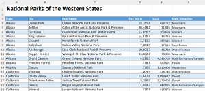
Figure 3.28 below shows a data set of some of the national parks of the Western States, including the park sizes, visitors in the year 2023, and main attractions. One question we might ask about this data set would be, What was the total number of visitors to these parks by state in the year 2023? To answer this question, we would have to sum up the number of visitors for the parks in each state, which could take a bit of time.
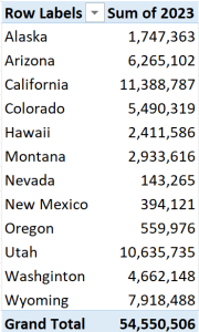
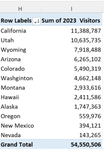
However, if we create a PivotTable from this data set, the answer to our question is immediately calculated and displayed in an easy-to-read table. It might look like the PivotTable in the image below. We say “might” because there are many ways you can create a PivotTable.
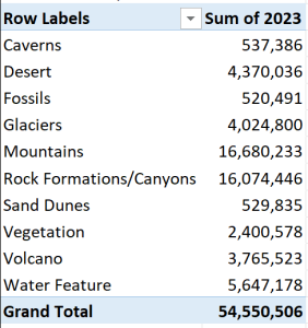
Not only are there many ways to create a PivotTable, you can also rearrange–or pivot–the information in a PivotTable to answer other questions or look at the data from a different perspective. Another question we could ask about the parks data would be, What were the total visitors by main attraction? To answer this question, we just need to change out the State data from the previous PivotTable to the Attraction data. This simply involves dropping and dragging or selecting and deselecting fields or data. Our adjusted PivotTable would look like this:
Let’s try it:
Open the “CH3-Gradebook and Parks” workbook if it isn’t already open.
Click on the “PivotTable” sheet tab within your “CH3-Gradebook and Parks” workbook.  .
.
On this spreadsheet is data about the national parks in the Western United States as shown in Figure 3.28 above. First, we’ll create the PivotTable in Figure 3.29 above, showing the total number of visitors to the parks by state for the year 2023.
- Select the cells (including column headers) you want to include in your PivotTable, we will select cells A3:F43.
- On the Insert tab click the PivotTable command. See Figure 3.31.
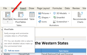
Figure 3.31 PivotTable Command on the Insert Tab - The PivotTable from table or range dialog box opens, Figure 3.32. You will choose your settings, then click OK. Since we already selected the range A3:F43, it populates into the Table/Range box. For this practice, we will place the PivotTable on our PivotTable sheet beginning in cell H3. Click on the radio button for “Existing Worksheet,” then your insertion point will move to the “Location:” box, then click on cell H3 of the PivotTable sheet. See Figure 3.32.
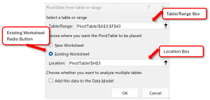
Figure 3.32 PivotTable from table or range dialog box. - A blank PivotTable in cell H3 and the Field List will appear on the worksheet. Figure 3.33.
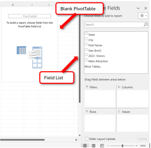
Figure 3.33 Blank PivotTable with Field List. - Once you create a PivotTable, you then decide which fields to use to build the PivotTable. Each field is a column header from the source data, and contain the data from that column. In the PivotTable Field List, check the box for each field you want to add, and Excel will populate that field into the area boxes beneath the field list. In our example, we want to know the total visits by each state, so we’ll check the State and 2023 Visitors fields. See Figure 3.34.
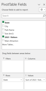
Figure 3.34 PivotTable Fields panel showing State and 2023 Visitor fields selected. - The PivotTable will calculate and summarize the selected fields. For our data set, the PivotTable shows the number of visitors by State. See Figure 3.35.
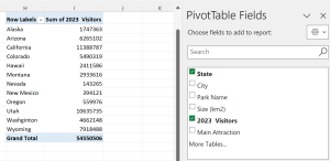
Figure 3.35 PivotTable Showing Park Visitors by State. - When you create a PivotTable, you get two new tabs on your ribbon specifically for working with your PivotTable, the PivotTable Analyze tab and the Design tab. See Figure 3.36.
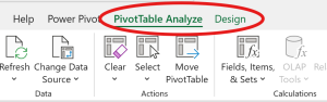
Figure 3.36 PivotTable Analyze and Design Tabs To change the number formatting for a PivotTable, go to the PivotTable Analyze tab, then the Active Field group, and click on “Field Settings.” See Figure 3.37.
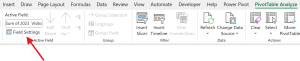
Figure 3.37 Field Settings Command for PivotTables In the Value Field Settings dialog box that opens, click on “Number Format” in the lower left corner, Figure 3.38, this will open up the Format Cells dialog box where you can set the number format.
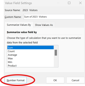
Figure 3.38 Number Format Button in the Value Field Settings Dialog Box We want to change the number format to “Number” with zero decimal places and use the 1000 Separator. Select these options, then click OK, then Ok again to set the number format. See Figure 3.39.
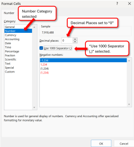
Figure 3.39 Format cells dialog box.
Our PivotTable with the numbers formatted:
Pivoting data
One of the powerful things about PivotTables is that they can quickly pivot—or reorganize—your information. This allows you to analyze your data in many ways, answering different questions and even discovering new trends and patterns.
To add columns:
Currently our PivotTable only shows one column of data. We can show multiple columns by adding a field to the Columns area.
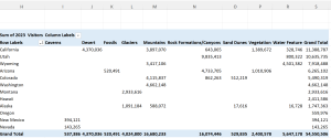
- Drag a field from the Field List into the Columns area. We’ll use the Main Attraction field. Click on the Main Attraction field in the fields list and drag it into the Columns area. See Figure 3.41.
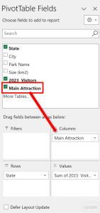
Figure 3.41 Main Attraction Field Moved to the Columns area in the PivotTable Fields Panel - The PivotTable now includes multiple columns. There is now a column for each of the main attractions in addition to the grand total, Figure 3.42. Now we can see which attractions seem to draw the most visitors.
To change a row or column:
You can also change a row or column in your PivotTable. This will give you a different analysis. You simply remove one field, by dragging it out or deselecting it, and select or drag in another field or fields.
- We’ll remove the Main Attraction and 2023 Visitors fields. Drag these fields out of their current areas. You can also uncheck the appropriate box in the Field List. See Figure 3.43.
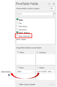
Figure 3.43 Removing fields - Drag a new field into the desired area. We will place the Park Name field in the Values area. By placing a text based field, such as Park Name, in the Values area, Excel will give us a count of the items, Figure 3.44, whereas when we place a value based field in the Values area the default calculation will be Sum. You can change the calculation by going to the Value Field settings as we did to change the number format.
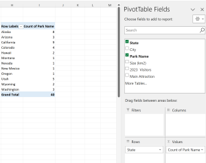
Figure 3.44 PivotTable showing count of parks. - You can also edit the column labels in a PivotTable so they are more descriptive under the Value Field Settings or by simply clicking in the cell and entering a new name. Click in cell H3 and type in the word “States,” then click in cell I3 and type in “#of Parks.” See Figure 3.45.
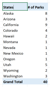
Figure 3.45 Column labels undated. As you can see, you can do a lot with PivotTables and they are a great tool.
- What other PivotTables could you make from the National Parks data set? Make another one or two PivotTables from the parks data set and place them on a new worksheet. Name the new sheet PivotTables. There is no one correct answer for this. Just give it a try!
