
4.2 Experiments and Probability of Events
Why Study Probability?
The use of statistics today relies on taking sample data from a population, then using that data to make an inference about the larger group. The study of probability (or chance) plays a major role here. Once a sample is determined, researchers must decide how likely that sample would be to occur. Different inferences would be made if the sample collected is quite likely or quite unlikely to occur.
You’ve seen this idea in magic tricks. When the performer “guesses” your card without having looked at it, the audience is amazed. The magician should only be able to guess your card randomly only 1 out of 52 times! But when the magician guesses your card correctly, we know that something extraordinary has happened, because it was unlikely.
The same would be true if you were working in public health. Officials usually have decades of data on disease rates, so they know what proportion of residents would have a cold on any given day. If officials were to take a random sample and see that the numbers are unusually high, then they may decide to take some action to combat the outbreak, such as social media announcements. However if the sample showed the expected number of colds, then the agency would likely not make the extra announcements.
You do this sort of probability based decision making all the time. Can you think of a time when you saw that something was unlikely and you made a decision as a result?
Probability Definition and Properties
The probability of any outcome is the long-term relative frequency of that outcome in the sample space, S (i.e. the set of all possible outcomes). See text below for more definitions.
- Probability refers to future events, and the notation P(event) is the probability the event occurs.
- A probability is a proportion and always takes on a value between 0 and 1, inclusive, so
0 P(event) 1, for any event.
 - If the probability of an event is zero, we write P(event) = 0. This means the event will not happen.
- If the probability of an event is one, then we write P(event) = 1. This means the event will happen for sure.
- If an experiment is conducted, at least one outcome in the sample space is guaranteed, so P(S) = 1.
Terminology of Probability
We need to come to an understanding of probability and how it is used in statistics. This understanding will be developed over the course of this entire class. For now, keep in mind that probability is a number that is associated with how certain we are of the outcomes of an experiment or activity. While the word “experiment” might bring up a vision of a laboratory with beakers and bubbling solutions, when we talk about an experiment, we mean something different. An experiment is a planned operation carried out under controlled conditions. Results of an experiment are not known before the experiment is conducted, so the outcome is uncertain.
A result of an experiment is called an outcome. If we make a list of all the possible outcomes for an experiment, we create the sample space. We typically are interested in a particular collection of the outcomes, so an event is any combination or subset of outcomes of an experiment.
The uppercase letter S is used to denote the sample space. Because the sample space is a list of all the outcomes that are possible, we need a compact way to denote the list. In mathematics, we use curly brackets to list sets, this is called set notation, so the sample space for an experiment would be given by S = {list of all outcomes}.
Upper case letters like A and B are typically used to represent events. Because an event is a collection or subset of the sample space, we will use set notation to list outcomes associated with events as well. Any event should be described in words first and then the outcomes that make up the event should be listed as A = {list of outcomes corresponding to the event}.
Example 1: Describing a Sample Space and Events
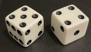
Craps is a dice game, which uses two six-sided dice, as shown in the photograph. When each die is rolled, the top face will show any of the number of dots: 1, 2, 3, 4, 5, or 6. Together the dice can show sums from 2 to 36. The most basic roll in craps is the “come out roll.” One player will roll the dice and the sum of the dice is observed. Some players will win if a 7 or 11 shows and lose if a 2, 3, or 12 shows. Consider the experiment of rolling the dice on the come out roll and create the following related to this experiment:
- Describe the experiment.
- Define the sample space and list the outcomes.
- Define event A as the winning roll and list the elements in event A.
- Define event B as the losing roll and list the elements in event B.
Answers:
- The experiment consists of rolling two six-sided dice and observing the sum of the dots (pips).
- The sample space consists of all of the possible outcomes when two dice are rolled. S = {2, 3, 4, 5, 6, 7, 8, 9, 10, 11, 12, 13, 14, 15, 16, 17, 18, 19, 20, 21, 22, 23, 24 25, 26, 27, 28, 29, 30, 31, 32, 33, 34, 35, 36}.
- Let event A = getting a 7 or 11; A = {7, 11}.
- Let event B = getting a 2, 3, or 12; B = {2, 3, 12}.
Combining Events
We often construct events by combining simpler events. All events are subsets of sample spaces, so we have seen how we use set notation to describe sample spaces and events. We can use set notation to combine sets as well.
The Union of two events,  , is the set of outcomes that belong to A, to B, or to both A and B at the same time. In words, “A or B” means the same thing as .
The Intersection of two events,  , is the set of outcomes that belong both to A and to B. In words, “A and B” means the same thing as .
The Compliment of an event A is the set of outcomes that are not in A, In words, “not A” means the same thing as A’.
- Union of Events: Sometimes we are interested in one event occurring or another event occurring. Event “A or B” will be made up of all outcomes in A, or in B, or in both A and B at the same time. We can describe this idea by using the word “or” but it is also common to use the union symbol,
 . Event “A or B” means the same thing as . For example, let A = {1, 2, 3, 4, 5} and B = {4, 5, 6, 7, 8}. If we create the event we will list the outcomes in A, or in B, or both A and B. In this case, = {1, 2, 3, 4, 5, 6, 7, 8}. Notice that 4 and 5 are NOT listed twice.
- Intersection of Events: Sometimes we are interested in two events occurring at the same time, so one event occurs and the other event occurs. We can describe this idea by using the word “and” but it is also common to use the intersection symbol,
 . Event “A and B” means the same thing as . For example, let A = {1, 2, 3, 4, 5} and B = {4, 5, 6, 7, 8}. Then = {4, 5}.
- Complement of an Event: Sometimes we are interested in outcomes that do not belong in an event A, so we are interested in what happens when A does not occur. The complement of event A is denoted A′ . We would read this as “A prime”. A′ consists of all outcomes that are not in A. An event and its compliment will not have outcomes in common and together would make up the entire sample space. For example, let S = {1, 2, 3, 4, 5, 6} and let A = {1, 2, 3, 4}. Then A’ = {5, 6}.
Example 2: Combining Events
An experiment is conducted in which we flip a two-sided coin (call one side “heads” (H) and the other side “tails” (T)), and then roll a six-sided die (sides are numbered 1 to 6).
Let event A = the number on the die is a 1 or 2. Let event B = the coin shows heads. We’ll denote the outcome of “rolling heads then roll a 1” will be denoted by “H1.”
Find each of the following:
- List S, A, and B using set notation.
- Find
- Find
- Create the sets A’, B’, and

Answers:
- S = {H1, H2, H3, H4, H5, H6, T1, T2, T3, T4, T5, T6}, A = {H1, H2, T1, T2}, B = {H1, H2, H3, H4, H5, H6}
- = {H1, H2, H3, H4, H5, H6, T1, T2}
- = {H1, H2}
- A’ = {H3, H4, H5, H6, T3, T4, T5, T6}, B’ = {T1, T2, T3, T4, T5, T6}, = {T3, T4, T5, T6}
Long Term Expectation and the Law of Large Numbers
There are situations in which the only way we can estimate a probability is to repeat the experiment many, many times and then calculate the proportion of times the event occurs. This important characteristic of probability experiments is known as the Law of Large Numbers which states that as the number of repetitions of an experiment is increased, the relative frequency obtained in the experiment tends to become closer and closer to the theoretical probability. Even though the outcomes do not happen according to any set pattern or order, overall, the long-term observed relative frequency will approach the theoretical probability. (The word empirical is often used instead of the word observed.)
For example, if you flip one coin six times, you could observe the outcome: H, H, H, H, H, T. On the other hand, you could observe the outcome H, T, H, T, H, T. What happens if you continue flipping and keep track of the number of heads you observe? Try it by going to the Coin Flip App to run a simulation.
We know in the long run, a fair coin will land heads up about 50% of the time, so does our coin flipping result contradict the theoretical probability? Not at all! Probability is not defined by what happens in the short term. However, if you repeatedly flip the coin, 20 times, 2000 times, 20,000 times, etc., the relative frequency of heads approaches 0.5, which is the true theoretical probability of heads occurring in the flip of a fair coin. P(head) = 0.5 means the event of observing a head in a future coin flip is equally likely to occur or not to occur. Equally likely means that each outcomes of an experiment occurs with equal probability. For example, if you toss a fair, six-sided die, each of the six faces (1, 2, 3, 4, 5, or 6) is as likely to occur as any other. If you toss a fair coin, a Head (H) and a Tail (T) are equally likely to occur. If you randomly guess the answer to a true/false question on an exam, you are equally likely to select a correct answer or an incorrect answer.
Probability of Equally-Likely Events
To calculate the probability of an event A when all outcomes in the sample space are equally likely, count the number of outcomes for event A and divide by the total number of outcomes in the sample space.

Example 3: Probability of Equally-Likely Events
- If you toss a fair dime and a fair nickel, list the outcomes in the sample space and calculate the probability of A, where A is the event of observing two heads.
- Suppose you roll one fair six-sided die, with the numbers {1, 2, 3, 4, 5, 6} on its faces. Let event E = rolling a number that is at least five. Calculate the probability of observing event E.
Answers:
- There are only four possible outcomes in the sample space, which can be listed as S = {HH, TH, HT, TT}, where T = tails and H = heads. Because both coins are fair, each of the four outcomes is just as likely to occur as the others. The event of observing two heads corresponds to outcome HH, which occurs exactly one time. There are four equally-likely outcomes in the sample space. Therefore,
 .
. - There are two outcomes {5, 6} that correspond to event E. Because the die is fair, each of the six sides has the same probability of being rolled. Therefore,
 .
.
It is important to realize that in many situations, the outcomes are not equally likely. A coin or die may be unfair, or biased. Two math professors in Europe had their statistics students test the Belgian one Euro coin and discovered that in 250 trials, a head was obtained 56% of the time and a tail was obtained 44% of the time. The data seem to show that the coin is not a fair coin; more repetitions would be helpful to draw a more accurate conclusion about such bias. Some dice may be biased. Look at the dice in a game you have at home; the spots on each face are usually small holes carved out and then painted to make the spots visible. Your dice may or may not be biased; it is possible that the outcomes may be affected by the slight weight differences due to the different numbers of holes in the faces. Gambling casinos make a lot of money depending on outcomes from rolling dice, so casino dice are made differently to eliminate bias. Casino dice have flat faces; the holes are completely filled with paint having the same density as the material that the dice are made out of so that each face is equally likely to occur. Later we will learn techniques to use to work with probabilities for events that are not equally likely.
Mutually Exclusive Events
Two events are mutually exclusive if they cannot both occur at the same time. The intersection of two mutually exclusive events would have no elements in it and would be empty. Any set that is empty is defined as the empty set. For example, we have already discussed the complement of an event. Any event and its complement would not share any elements, so they would be mutually exclusive. If we are curious about the probability of two mutually exclusive events happening, then we can add their probabilities.
Finding probabilities for events that are not mutually exclusive requires more care. If we just add the individual probabilities, then we are double counting probability where the two events share elements. Double counting occurs where the two events overlap. To correct for this issue, we can add the probabilities of the individual events as long as we subtract the probability where the intersection occurs. This brings us to several formulas for finding probabilities of combinations of events.
The Empty Set is a set with no outcomes: Empty Set = { } or  .
.
Two sets with no outcomes in common are called Mutually Exclusive, or disjoint.
Probabilities of Combinations of Events
If A and B are Mutually Exclusive Events:


If A and B are not Mutually Exclusive Events:
 . Note: For events that are not mutually exclusive, we will count twice any outcome that is a member of both events A and B, so we must take care to subtract the probability related to the intersection of A and B.
For an event A and its Complimentary Event A’ .


Example 4: Probability of Combinations of Events
A random number generator will produce a whole number between 1 and 19, inclusive. An experiment consists of generating one random number.
- List the sample space for the experiment.
- If event A = the number is even and event B = the number is greater than 13, then list elements in each event.
- Find the individual probabilities of event A and event B.
- List the elements in
 and list the elements in .
 - Find
 and
and  .
. - List the elements in A′ and find P(A′ ).
- P(A) + P(A′ ) =
Answers:
- S = {1, 2, 3, 4, 5, 6, 7, 8, 9, 10, 11, 12, 13, 14, 15, 16, 17, 18, 19}
- A = {2, 4, 6, 8, 10, 12, 14, 16, 18}, B = {14, 15, 16, 17, 18, 19}

- = {14, 16, 18}, = {2, 4, 6, 8, 10, 12, 14, 15, 16, 17, 18, 19}

- A′ = {1, 3, 5, 7, 9, 11, 13, 15, 17, 19};

- P(A)+P(A’)=

Example 5: Probabilities of Combinations of Events
Consider the experiment where we flip two fair coins. If we let events T = observe a tail and H = observe a head, then the possible outcomes of this experiment are HH, HT, TH, and TT . The sample space is {HH, HT, TH, TT}. Note, the outcomes HT and TH are different. The HT means that the first coin showed heads and the second coin showed tails. The TH means that the first coin showed tails and the second coin showed heads.
- Find the probability of getting at most one tail.
- Find the probability of getting all tails.
- Find the probability of getting all heads.
- Find the probability of getting more than one tail.
- Find the probability of getting a head on the first roll.
- Find the probability of getting at least one tail.
Answers:
- Let A = the event of getting at most one tail. (At most one tail means zero or one tail.) Then A can be written as {HH, HT,TH }. The outcome HH shows zero tails. HT and TH each show one tail. The probability for A is found as
 .
. - Let B = the event of getting all tails. B can be written as {TT }. B is the complement of A, so B = A′. Also, P(A) + P(B) = P(A) + P(A′ ) = 1. The probability for B is found as

- Let C = the event of getting all heads. C = {HH }. Since B = {TT }, P(B C) = ∅. Events B and C are mutually exclusive, as B and C have no elements in common because you cannot have all tails and all heads at the same time.
- Let D = the event of getting more than one tail. D = {TT }.
 .
. - Let E = the event of getting a head on the first roll. (This implies you can get either a head or tail on the second roll.) E = {HT, HH }.
 .
. - Find the probability of getting at least one (one or two) tail in two flips. Let F = event of getting at least one tail in two flips. F = {HT, TH, TT }.

Example 6: Probability of Mutually Exclusive Events
The U.S. Census Bureau surveyed 100,000 households where 305,688 people lived. The Census Bureau wanted to get social and economic information about people living in the United States. The two-way table below summarizes the people by the region of their primary residence in the United States who had no health insurance and also those who have some type of health insurance.
| Region | No Health Insurance | Some Health Insurance | Total |
| Northeast | 6761 | 47,957 | 54,718 |
| Midwest | 8598 | 57,408 | 66,006 |
| South | 21,639 | 91,498 | 113,137 |
| West | 12,837 | 58,990 | 71,827 |
| Total | 49,835 | 255,853 | 305,688 |
- Are the events “living in the South” and “living in the Midwest” mutually exclusive? Explain.
- Find the probability that a randomly selected person lives in the South or lives in the Midwest.
- Are the events “living in the South” and “having no health insurance” mutually exclusive? Explain.
- Find the probability that a randomly selected person lives in the South or has no health insurance. This probability can be represented as P(South or No Health Insurance). Write your answer as a decimal, rounded to two decimal places.
Answers:
- The events are mutually exclusive because no one can live in two regions at the same time. The events would have no elements in common.
- If we label the events as S = living in the South and M = living in the Midwest, then find P(S M) = P(S) + P(M). Using the table values, we see P(S M) =
 =
=  .
. - The events are not mutually exclusive. It is possible for a person who is living in the South to not have health insurance. Notice in the table, there are 21,639 people who live in the South and who do not have health insurance. If two events can share elements, then the events are not mutually exclusive.
- If we label the events as S = living in the South and N = having no health insurance, then find P(S N) = P(S) + P(N) – P(S N). Using the table values, we see P(S N) =
 =
=  .
.
In the previous example, the information about region and health insurance were presented in a table. A contingency table provides a way of portraying data that can facilitate calculating probabilities. The table helps in determining conditional probabilities quite easily. The table displays sample values in relation to two different variables that may be dependent or contingent on one another.
Example 7: Using a Contingency Table
Texting and driving is a risky behavior. According to the National Highway Traffic Safety Administration (NHTSA), driving at a rate of 55 miles per hour while sending or reading a text message for five seconds is the same as driving the entire length of a football field with your eyes shut.1 Suppose data was collected at an intersection in a small town and, over the course of a week, 755 cars were observed passing through the intersection. The contingency table summarizes fictitious data about the drivers who were or were not using a cell phone and whether or not they were speeding.
| Speeding | Not Speeding | Total | |
| Using A Cell Phone | 25 | 280 | 305 |
| Not Using A Cell Phone | 45 | 405 | 450 |
| Total | 70 | 685 | 755 |
Looking over the table, we see 305 drivers who passed through the intersection used a cell phone and 25 of them were speeding. Of the 450 drivers who were not using a cell phone, 45 of them were speeding.
Calculate the following probabilities using the information from the table.
- Find P(Using a Cell Phone).
- Find P(Speeding).
- Find P(Using a Cell Phone AND Speeding) = P(Using a Cell Phone Speeding).
- Find P(Using a Cell Phone OR Speeding) =P(Using a Cell Phone Speeding).
Answers:
-
- P(Using a Cell Phone) =

- P(Speeding) =

- P(Using a Cell Phone
 Speeding) =
- P(Using a Cell Phone Speeding)
= P(Using a Cell Phone) + P(Speeding) – P(Using a Cell Phone Speeding)
=
- P(Using a Cell Phone) =
Videos
This YouTube video gives more examples of basic probabilities: Introduction to Probability
This YouTube video gives examples of probabilities involving AND.
This YouTube video gives examples of probabilities involving OR.
This YouTube video gives examples of finding probabilities related to mutually exclusive events.
This YouTube video gives an example of finding probabilities using a contingency table.
Sources
Example 4 was used from Statway College Module 2, by Carnegie Math Pathways is licensed under CC BY NC 4.0.
1NHTSA “Distracted Driving”. Available online at https://www.nhtsa.gov/risky-driving/distracted-driving (accessed 3/14/20240
To make a generalization about a population using only sample data
A process that results in an outcome that cannot be predicted in advance with certainty.
The result of an experiment.
The set of all possible outcomes of an experiment.
Any combination of outcomes of an experiment. It is also a subset of a sample space.
A set with containing no outcomes. It is a set with nothing inside, so we use { }.
Events that cannot both occur at the same time.
A display of data in rows and columns for two different variables.

Feedback/Errata