
6.2 Continuous Probability Density Functions
California suffers from poor air quality, especially in the San Joaquin Valley, for nonattainment of the federal ozone standard of 70 parts per billion. In California and many other states, part of the plan to address issues like these involves imposing zero-emission vehicle registration. Cars must get as close as possible to zero emissions and California is moving to accelerate to 100% new zero-emission vehicle sales by the year 2035. Emission measurements taken from automobiles are not discrete values, as measurements are not taken from a discretely spaced set of numbers. Auto emissions measure such things as carbon monoxide, hydrocarbon, carbon dioxide, and oxygen levels. Consider the random variable X = level of carbon dioxide produced in grams per gallon of gasoline. A measurement like this can be measured to any degree of accuracy and takes on values along a continuous interval. This is one example of a continuous random variable. Unlike discrete random variables, we cannot make a table and list all the possible values that the random variable can take on. We cannot add up discrete probabilities to describe the probability the random variable takes on a specific value or range of values. Continuous random variables require a different treatment.
Probability Density Function
A continuous random variable is one in which probabilities are represented by areas under a curve. The curve is called the probability density function, PDF, or the probability distribution. We use the probability density function f (x) to draw the graph of the probability distribution. Because the probability density function is a curve, the areas between the curve and the horizontal axis represent probabilities, so the total area must be one, and must be found using integral calculus, geometry, or approximation techniques. See Figure 1 (a).
The area under the probability density curve between two points corresponds to the probability that the variable falls between those two values. In other words, the area under the density curve between points a and b is equal to  . See Figure 1 (b).

Probability Density Function of a Continuous Random Variable
A Probability Density Function, PDF, of a continuous random variable X is a function  on a domain S that satisfies the following properties:
 for all

So for any subset  ,
,  .
.
Properties of Continuous Probability Distributions
- The entire area under the probability density function curve and above the x-axis is equal to one.
 .
. - Probability is found for intervals of x values rather than for individual x values.
 is the probability that the random variable X takes on values in the interval between the values c and d, so
  .
. - The probability that x takes on any single individual value is zero.
 , so
, so  .
. - There is no area added when you include the endpoints of the interval.
 is the same as
  .
.
We will find the areas that represents probability by using geometry or integral calculus. There are many continuous probability distributions. When using a continuous probability distribution to model probability, the particular distribution function used is selected to model and fit the particular situation in the best way. In this chapter, we will study several continuous probability distributions.
Example 1 – Probabilities for a Continuous Random Variable
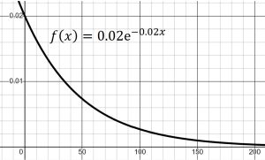
Family-car tires can last 70,000 miles or more according to Consumer Reports from April 2022. Many all-season light trucks and SUV tires can last longer, however, it was found that ultra-high-performance tires generally do not last as long. Many summer tires do not even carry warranties! Suppose engineers have developed a new tire with lifetimes (in thousands of miles) given by the following probability density function, f(x).  , for x > 0. The continuous random variable X = the lifetime in thousands of miles for a tire.
(a) Verify this is a PDF.
(b) Find the probability a tire lasts up to 100,000 miles.
(c) Find the probability a tire lasts between 100,000 miles and 150,000 miles.
Solutions:
(a) Integrate the PDF on its domain and show the area is equal to one.
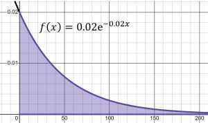 Since this function has an elementary antiderivative, we can integrate directly over the entire domain.
![\begin{align*} P(x \geq 0) &= \int_{0}^{\infty} 0.02e^{-0.02x}dx \\ &=\lim_{t \rightarrow \infty}\int_{0}^{t} 0.02e^{-0.02x}dx \\ &=\lim_{t \rightarrow \infty}[-e^{-0.02t}+e^0] \\ &=1 \end{align*}](https://openoregon.pressbooks.pub/app/uploads/quicklatex/quicklatex.com-efe2e21d6cbbc3a26a1a11cb9270b6cf_l3.png "Rendered by QuickLaTeX.com")
(b) To find the probability a tire lasts up to 100,000 miles, find  . The probability is shown in the shaded area below.
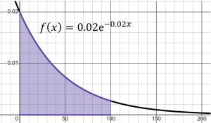
![\begin{align*} P(0 \leq x \leq 100) &= \int_{0}^{100} 0.02 e^{-0.02 x} dx \\ &= \left[ -e^{-2} + e^0 \right] \\ &\approx 0.86 \end{align*}](https://openoregon.pressbooks.pub/app/uploads/quicklatex/quicklatex.com-f5c47dc1617e0682af5453eaf53a7d84_l3.png "Rendered by QuickLaTeX.com")
(c) To find the probability a tire lasts between 100,000 miles and 150,000 miles, find  . The probability is shown in the shaded area below.
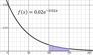
![\begin{align*} P(100 \leq x \leq 150) &= \int_{100}^{150} 0.02e^{-0.02x}dx \\ &= \left[ -e^{-3}+e^{-2} \right] \\ &\approx 0.086 \end{align*}](https://openoregon.pressbooks.pub/app/uploads/quicklatex/quicklatex.com-0022277bb34478ca9e06b81181c44030_l3.png "Rendered by QuickLaTeX.com")
Approximately 8.6% of tires will last between 100,000 miles and 150,000 miles.
Mean and Variance of a Continuous Random Variable
There are parallels between how we find the mean and variance of a continuous random variable compared to a discrete random variable. Recall when finding the mean of a discrete random variable, each value the random variable can take on is weighted (multiplied) by its probability before adding. With continuous random variables, probabilities are described using the probability density function and we use integration. The mean is defined to be the center of mass of its probability density function and the variance is the moment of inertia around the vertical axis through the population mean. Both of these ideas are defined as integrals.
The mean is often called the expected value of X and is also often denoted as E(X),  , or most often simply by
  . The variance is often denoted as V(X),
  , or most often simply by
  Also note that the standard deviation is the square root of the variance.
Definitions: Mean and Variance of Continuous Random Variables
If X is a continuous random variable with probability density function, , then
The mean of X is given by 
The variance of X is given by 
An equivalent, and often more convenient formula for the variance is given by 
Example 2 – Mean, Variance, and Standard Deviation Calculation
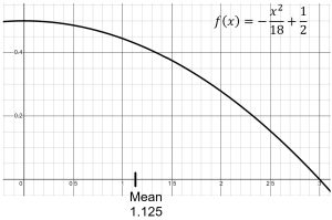
Projectiles are fired at a circular target which has a 3 meter radius. The distance in meters from the point of impact to the center of the target is a continuous random variable, X. The PDF is given by  , where
(a) Find the mean of the random variable.
(b) Find the variance and standard deviation of the random variable.
(c) Find the probability the impact is less than one standard deviation from the center fo the target.
Solutions:
(a) To find the mean,  , we use the integral from the definition above:
![\begin{align*} \mu_{X} &= \int_{0}^{3} x \left( -\frac{x^2}{18} + \frac{1}{2} \right) \enspace dx \\ &= \int_{0}^{3} -\frac{x^3}{18}+\frac{x}{2} \enspace dx \\ &= \left[-\frac{x^4}{72}+\frac{x^2}{4}\right]_{0}^{3} \\ & = 1.125 \text{ meters} \end{align*}](https://openoregon.pressbooks.pub/app/uploads/quicklatex/quicklatex.com-a9ff4c57caa82da8f8c24ce36770f206_l3.png "Rendered by QuickLaTeX.com")
Thus, the mean of the random variable is 
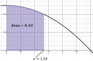
(b) To find the variance of the random variable, we use the integral from the definition above:
![\begin{align*} \sigma^2_X &= \int_0^3 x^2 \left( -\frac{x^2}{18} + \frac{1}{2} \right) dx - \mu^2 \\ &= \int_0^3 \left( -\frac{x^4}{18} + \frac{x^2}{2} \right) dx - 1.125^2 \\ &= \left[ -\frac{x^5}{90} + \frac{x^3}{6} \right]_0^3 - 1.125^2 \\ &= 1.8 - 1.125^2 \\ &\approx 0.534 \text{ square meters} \end{align*}](https://openoregon.pressbooks.pub/app/uploads/quicklatex/quicklatex.com-92170d2d02401cab4e267c3467dd495d_l3.png "Rendered by QuickLaTeX.com")
Thus the variance of the random variable is  Further, the standard deviation of the random variable is
(c) To find the probability that the impact is less than one standard deviation from the center, we must compute  .
.
![\begin{align*} P( 0 < x < 0.731 ) &= \int_0^{0.731} \left( -\frac{x^2}{18} + \frac{1}{2} \right) dx \\ &= \left[ -\frac{x^3}{54} + \frac{x}{2} \right]_0^{0.731} \\ &\approx 0.3583 \end{align*}](https://openoregon.pressbooks.pub/app/uploads/quicklatex/quicklatex.com-3fc922b107b55309a8d584c3c4996160_l3.png "Rendered by QuickLaTeX.com")
So, approximately 36% of the projectiles will hit the target within one standard deviation of the center. (The graphic below is not correct.)
Cumulative Distribution Function
For a continuous random variable, X, the cumulative distribution function is created by adding probabilities up to a specified value. With a discrete probability distribution, we could add up individual probability values from a table, but for continuous random variables, adding up probabilities requires integral calculus. Often the cumulative distribution function can be found using integral calculus and then the function generated can be used for future needs. In other cases, when integration is impossible, probabilities are calculated by approximation. When we use formulas related to continuous probability distributions later, keep in mind the formulas were originally found by using the techniques of integral calculus.
Definition: Cumulative Distribution Function for a Continuous Random Variable
The Cumulative Distribution Function, CDF, of a continuous random variable X is  .
.

Where  is the probability density function
Example 2 – Finding the Cumulative Distribution Function
Use the new tire probability density function from Example 1, , for x > 0, and find each of the following.
(a) Create the cumulative distribution function.
(b) Use the cumulative distribution function to find the probabilities a tire will last up to 10,000 miles; 40,000 miles; 80,000 miles; 120,000 miles; and 200,000 miles.
Solutions:
(a) ![F(x)=P(X \leq x) = \int_{0}^{x} 0.02e^{-0.02t}dt=[ -e^{-0.02t}]_0^x=-e^{-0.02x}+1.](https://openoregon.pressbooks.pub/app/uploads/quicklatex/quicklatex.com-88db70d1e118e7a5d4b5618887dbeabb_l3.png "Rendered by QuickLaTeX.com")
(b) Now that we have the cumulative distribution function we can input any value of the random variable and it will give the probability of a tire lasting up to that many miles. Remember that for this model, miles is in thousands.
 , so approximately 18% of tires will last up to 10,000 miles.
 , so approximately 55% of tires will last up to 40,000 miles.
 , so approximately 80% of tires will last up to 80,000 miles.
 , so approximately 91% of tires will last up to 120,000 miles.
 , so approximately 98% of tires will last up to 200,000 miles.
Sources
California Air Resources Board. (2024, June 12). Zero-Emission Vehicle Program. CA.gov. https://ww2.arb.ca.gov/our-work/programs/zero-emission-vehicle-program
CR Consumer Reports. (2022, April 4) Gene Peterson. How long do Tires Last? Consumer Reports’ Treadwear Testing Will Tell You. https://www.consumerreports.org/cars/tires/how-long-do-tires-last-consumer-reports-treadwear-testing-a5353952733/.

Feedback/Errata