
6.4 The Exponential Distribution
The exponential distribution is often (but not always) concerned with the amount of time until some specific event occurs, so it is a continuous distribution. For example, the amount of time (beginning now) until an earthquake occurs has an exponential distribution. Other examples include the length of time of a business telephone call, and the amount of time a car battery lasts.
Fewer values for an exponential random variable tend to be larger, while typically there are more small values, so it is a skewed distribution. For example, the amount of money spent in a shopping trip follows an exponential distribution. There are more people who spend small amounts of money and fewer people who spend large amounts of money. The exponential distribution is widely used in the field of reliability. Reliability deals with the amount of time a product or component lasts. Because of this, the exponential distribution is often called the waiting time distribution. There is also a connection between the exponential and Poisson distributions.
Exponential Probability Distribution
If the random variable  , the probability density function
  is skewed and the shape of the density function depends on the parameter
  . Because the random variable
  is a measure of time, it must be greater than zero.
The exponential probability density function is  .
.
Calculating probabilities associated with the exponential distribution requires a substitution method. Rather than carry out an integration for each probability calculation, integration can be used once to create a cumulative function, which can then be used to calculate probabilities.
The cumulative distribution is found as  After integrating we find the cumulative distribution function is
  for
for 
To derive the mean, we must integrate  . Note that it is an improper integral and integration by parts is needed to integrate. To derive the variance, we must integrate
  . Note that it is also an improper integral and integration by parts is needed twice to integrate. Both integrations are well within your abilities and you are encouraged to derive them.
The mean of the exponential random variable,  .
.
The variance of the exponential random variable 
These details are summarized next.
Exponential Probability Density Function
For ,
The PDF is  for
for
The CDF is for
Mean: 
Variance: 
Standard Deviation: 
Example 1 – Time With a Patient
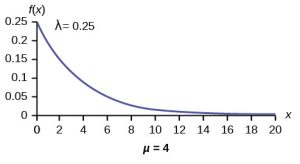
Let X = amount of time (in minutes) a health-care receptionist spends with a patient. The time is known to have an exponential distribution with the mean of four minutes.
- Create the PDF and find the mean and standard deviation.
- What is the probability the receptionist will spend at most 2 minutes with a patient?
- What is the probability the receptionist will spend more than 10 minutes with a patient?
Solutions:
(1)
We know the mean of the exponential distribution,  = 4 minutes. To write the PDF, we must determine the value of the parameter . Since
  , we can see that
  . Therefore, in this situation,
  . Hence, the distribution of this exponential random variable is
  . Further, the PDF is
  and is graphed below. Note the standard deviation,
  , is the same as the mean in this case, thus
  minutes.
(2)
To find the probability the receptionist will spend at most 2 minutes with a patient, use the CDF. Find  . Thus, about 40% of the time the receptionist will spent at most 2 minutes with a patient.
(3)
To find the probability the receptionist will spend at more than 10 minutes with a patient, find  . There is approximately an 8.2% chance the receptionist will spend more than 10 minutes with a patient.
The Relationship Between the Exponential and Poisson Distributions
You might recall, when we studied the discrete Poisson random variable, we used the parameter to represent the mean number of events in a given time. It is no accident that we use the parameter while discussing the continuous exponential distribution. When the underlying process is Poisson, with a fixed mean rate involving events per unit time, the exponential random variable has a mean,  , so the mean is the average time until the next event.
Example 2 – Time Until Next Geyser Eruption
Yellowstone National Park contains over half of the world’s geysers. A geyser is a hot water vent in the earth’s surface. Visit the Current Geyser Activity webpage. A geyser erupts on average every 8 minutes. The amount of time until the next eruption can be modeled by an exponential distribution with the average amount of time equal to 8 minutes. Write the distribution, state the probability density function, and graph the distribution. Then find the probability that it takes the geyser between four and five minutes to erupt.
Solutions:
If we let  the time in minutes until the next eruption, then
  = 8 minutes, so
  . Thus,
  , and the PDF is
  .
.
The probability it takes the geyser between four and five minutes to erupt is given by the following:

Approximately 7% of the time it will take between 4 and 5 minutes for the geyser to erupt.
Example 3 – Airline Ticket Purchase
The number of days ahead travelers purchase their airline tickets can be modeled by an exponential distribution with the average amount of time equal to 15 days.
- Find the probability that a traveler will purchase a ticket fewer than ten days in advance.
- How many days do 90% of all travelers wait?
Solutions:
If we let the number of days ahead travelers purchase their airline tickets, then  . Since the average amount of time is 15 days, we know that
  . The probability density function for this example is then
  .
.
(1)
The probability that a traveler will purchase a ticket fewer than ten days in advanced is  .
.

Therefore, approximately 49% of travelers will purchase a ticket fewer than ten days in advance.
(2)
When we want to find the number of days for which 90% of travelers wait, we can use the CDF and solve the following equation (see note below):


We conclude that 90% of travelers buy tickets fewer than 34.54 days in advance.
Note on the use the PDF and CDF
In the above example, we could use direct integration because the PDF of a random variable with an exponential distribution has an elementary antiderivative. This will not be true in most cases.
In most cases, students will make use of statistical software to find probabilities and percentiles. Students should NOT spend much time on antidifferentiation, and should instead learn to use the statistical software package of their choice.
Example 4 – Component Life
A quality control engineer collected data to assess how long a certain electronic component lasts. On the average, it was determined that the electronic component lasts ten years. If we assume this average is fixed, then the length of time the component lasts is exponentially distributed.
- What is the probability that a component lasts more than 7 years?
- Find the 80th percentile and explain its meaning.
- What is the probability that a component lasts between nine and 11 years?
Solutions:
(1)
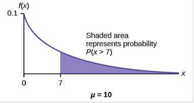
Let the random variable the amount of time (in years) a component lasts. We know  10 years, so
  . Therefore,
  . The following graph shows the shaded area under the PDF that represents the probability
  .
.
 To calculate this probability, we write
  . We can use the CDF
  , so
, so  . The probability that a component lasts more than seven years is 0.4966 or about 49.7% of components last more than 7 years.
(2)
To find the 80th percentile, we can use the CDF again as follows:

Eighty percent of components last at most 16.1 years.
(3)
What is the probability that a component lasts between nine and 11 years?

Approximately 7.4% of components will last between nine and 11 years.
Example 5 – Time Between Events
The time spent waiting between events is often modeled using the exponential distribution. For example, suppose that an average of 30 customers per hour arrive at a store and the time between arrivals is exponentially distributed.
- On average, how many minutes elapse between two successive arrivals?
- After a customer arrives, find the probability that it takes less than one minute for the next customer to arrive.
- After a customer arrives, find the probability that it takes more than five minutes for the next customer to arrive.
- Is an exponential distribution reasonable for this situation?
Solutions:
- Since we expect 30 customers to arrive per hour (60 minutes), we expect on average one customer to arrive every two minutes on average, so
 minutes between arrivals.
 - Let X = the time between arrivals, in minutes. , so
 = 0.5.
Therefore, . Calculate
  . About 39% of the time it will take less than one minute for the next customer to arrive.
 - Calculate
 . Approximately 8% of the time it will take more than five minutes for the next customer to arrive.
 - This model assumes that a single customer arrives at a time, which may not be reasonable since people might shop in groups, leading to several customers arriving at the same time. It also assumes that the flow of customers does not change throughout the day, which is not valid if some times of the day are busier than others. We can use the exponential distribution to give probabilities as long as we understand the limitations.
Memoryless Property of the Exponential Distribution
In Example 1, recall that the amount of time between patients is exponentially distributed with a mean of two minutes, X ~ Exp(0.5). Suppose that five minutes have elapsed since the last customer arrived. Since an unusually long amount of time has now elapsed, it would seem to be more likely for a customer to arrive within the next minute. With the exponential distribution, this is not the case. The additional time spent waiting for the next customer does not depend on how much time has already elapsed since the last customer. This is referred to as the memoryless property. Specifically, the memoryless property says that the probability of waiting a certain amount of time given that we know how long the last waiting time was, is exactly the same as if we did not know how long the last waiting time was.
The exponential distribution is often used to model the longevity of an electrical or mechanical device. In Example 4, the lifetime of a certain component has the exponential distribution with a mean of ten years, X ~ Exp(0.1). The memoryless property says that knowledge of what has occurred in the past has no effect on future probabilities. In this case, it means that an old part is not any more likely to break down at any particular time than a brand new part. The part stays as good as new until it suddenly breaks, so if the part has already lasted ten years, then the probability that it lasts another seven years is the same as the probability a new component lasts for seven years.
More on the Relationship between the Poisson and the Exponential Distribution
There is an interesting relationship between the exponential distribution and the Poisson distribution. Suppose that the time that elapses between two successive events follows the exponential distribution with a mean of units of time. Also assume that these times are independent, meaning that the time between events is not affected by the times between previous events. If these assumptions hold, then the number of events per unit time follows a Poisson distribution with mean. Recall that if X has the Poisson distribution with mean , then  . Conversely, if the number of events per unit time follows a Poisson distribution, then the amount of time between events follows the exponential distribution.
Example 6 – Time Between Calls
At a police station in a large city, calls come in at an average rate of four calls per minute. Assume that the time that elapses from one call to the next has the exponential distribution. Take note that we are concerned only with the rate at which calls come in, and we are ignoring the time spent on the phone. We must also assume that the times spent between calls are independent. This means that a particularly long delay between two calls does not mean that there will be a shorter waiting period for the next call. We may then deduce that the total number of calls received during a time period has the Poisson distribution.
- Find the average time between two successive calls.
- Find the probability that after a call is received, the next call occurs in less than ten seconds.
- Find the probability that exactly five calls occur within a minute.
- Find the probability that less than five calls occur within a minute.
- Find the probability that more than 40 calls occur in an eight-minute period.
Answers:
- On average there are four calls per minute, so
 calls per minute. The average time between calls is
  minutes between calls.
 - The fact that a call has been received is independent of the time it takes until the next call is received. Let T = time elapsed between calls. We know
 and
and  . Thus,
  . Ten seconds is
  of a minute, so
  . We predict that roughly 49% of the time the next call will occur in less than 10 seconds.
 - Let the number of calls per minute. The number of calls per minute has a Poisson distribution, with a mean of four calls per minute. Therefore,
 , and
, and  0.1563.
 - Keep in mind that X must be a whole number, so the whole number less than 5 is 4 and
 .
To compute this, we could take
.
To compute this, we could take .
. -
Let Y = the number of calls that occur during an eight minute period.Since there is an average of four calls per minute, there is an average of (8)(4) = 32 calls during each eight minute period.Hence,
 . Therefore,
  .
.
Sources
Current geyser activity – Yellowstone National Park (U.S. National Park Service). (n.d.). https://www.nps.gov/yell/planyourvisit/geyser-activity.htm

Feedback/Errata