7.3 Sampling Distribution and the Central Limit Theorem

Jeff Crabill; Vikki Maurer

7.3 Sampling Distribution and the Central Limit Theorem

So far, we have studied various distributions, both discrete and continuous, of random variables and learned that the data takes on a shape, also called a distribution. In this section, we will extend that same idea to individual statistics. When we take a sample from a population, we get one of sample out of possibly an infinite number of samples. Once we have the sample, we use summary statistics, such as the sample mean to help describe the sample and make generalizations about the population from which the sample was drawn. The sample mean is just one of the many sample means we could have observed. If we create a histogram of the sample means, we can see the distribution of the sample means. Every statistic has its own distribution, called the sampling distribution. How does the sampling distribution of the sample mean behave? What does it look like? Why do we care? As we will see, these questions form some of the most important questions and implications in statistics.

Key Idea

Every statistic has a sampling distribution! We can estimate the sampling distribution by taking random samples of size n and creating a histogram with the statistic generated from each sample. The more samples we take, the more our sampling distribution will reflect the theoretical distribution of the statistic.

Sampling Distribution of a Statistic

Just like data has a distribution, so does a statistic. Earlier in the course, you created histograms by collecting the data into groups and identifying the frequency of the data to construct the histogram. In the same way, we can take a random sample and record a statistic. After we do that hundreds of times, we will generate hundreds of data points (each one is a value of the statistic), and thus create a histogram. That histogram shows the sampling distribution of the statistic.

Example 1 – Sampling Distribution of a Sample Mean

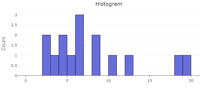
Let’s consider a small data set, which will be our population. Notice the population contains a total of 15 values. Because we have the entire population, we can calculate the population mean to be 7.53 and the standard deviation to be 5.26, so $\mu = 7.53$ and $\sigma = 5.26$ . Create a histogram of the population and then use a statistical program to draw 1100 samples of size 4 and create a histogram of the 1100 sample means.

Population, X = {2, 10, 5, 8, 8, 6, 3, 4, 18, 12, 2, 6, 4, 6, 19}

Solution:

Histogram of the original population, — Figure 1: Population Histogram

To estimate the sampling distribution, we take 1100 samples of size 4 and calculate the mean of each:

Sample 1: {12, 3, 6, 5} $\bar{x}_1 = 6.5$
Sample 2: {18, 12, 6, 6} $\bar{x}_2 = 10.5$
Repeat this process a total of 1100 times and create a histogram.

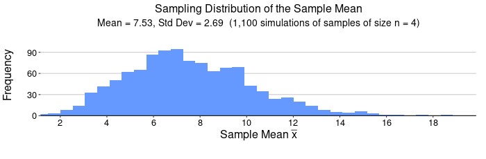
Sampling Distribution of 1000 sample means generated from the original population. The histogram appears to be symmetric and somewhat bell shaped. — Figure 2: Sampling Distribution of Sample Means

This histogram generated in Figure 2 is called a sampling distribution of the statistic $\bar{x}$ . The statistical program that gave the histogram also generated the mean of the sampling distribution and the standard deviation of the sampling distribution, called the standard error. Notice that the mean of the sampling distribution is the SAME as the mean of the population! Also notice that the standard error is SMALLER than the standard deviation of the population. In this case the sampling distribution has a standard error that is about half of the population standard deviation.

The Central Limit Theorem

This brings us to a critical and powerful theorem in statistics, the Central Limit Theorem.

The Central Limit Theorem is one of the most useful ideas in all of statistics. There are two alternative forms of the theorem, and both alternatives are concerned with drawing finite samples size n from a population with mean, $\mu$ and standard deviation, $\sigma$ .

The first alternative says that if we collect samples of size n, with a large enough n, calculate the mean of each sample, and create a histogram of those means, then the resulting histogram will tend to have an approximate normal distribution.
The second alternative says that if we collect samples of size n, with a large enough n, calculate the sum of each sample and create a histogram, then the resulting histogram will again tend to have a normal distribution.

In either case, it does not matter what the distribution of the original population is at all! The important fact is that the distribution of sample means and the distribution of sample sums tend to follow the normal distribution. For what we are doing, we will concentrate on what the Central Limit Theorem states as it concerns the sample mean.

The size of the sample, n, that is required in order to be “large enough” depends on the original population from which the samples are drawn (the sample size should be at least 30 or the data should come from a normal distribution). If the original population is far from normal, then more observations are needed for the sample means or sums to be normal. Sampling is done with replacement.

Central Limit Theorem

Random variable X has mean $\mu$ and standard deviation $\sigma$ .

For sufficiently large sample sizes, the random variable $\bar{X}$ has a normal distribution with the following mean and standard error:

$\mu_{\bar{X}} = \mu$
$\sigma_{\bar{X}} = \dfrac{\sigma}{\sqrt{n}}$

For any random variable X, $\bar{X} \sim N \left( \mu, \dfrac{\sigma}{\sqrt{n}} \right)$ if the sample size is sufficiently large.

If $X \sim N(\mu,\sigma)$ , then $\bar{X} \sim N \left( \mu, \dfrac{\sigma}{\sqrt{n}} \right)$ regardless of the sample size.

The Central Limit Theorem tells us that if we take large enough samples, then we do not need to know the underlying population distribution. We will be able to assume the sample means will have a normal distribution with a known mean and a known standard deviation (standard error). Moreover, looking closely at the standard deviation of the sample mean (standard error) it is clear that sample size has a big effect on the variability of the sample mean. With larger samples, we can expect less variability in $\bar{x}$ , which is a very useful fact in data science. Not it makes perfect sense why, in Example 1, we noted that the standard error was about half compared to the population standard deviation. Our sample size was 4 and the square root of 4 is 2, so the Central Limit Theorem predicted the standard error of the sample mean would be $\sigma/2$ .

Standard Error

The value $latex \sigma_{\bar{X}} = \dfrac{\sigma}{\sqrt{n}} $ is also known as the standard error of the mean.

Sampling Distribution of the Sample Mean, $\Huge\bar{x}$

Why are we so concerned with means? Just two reasons are that they give us a middle ground for comparison, and they are easy to calculate. Now that we are aware of the Central Limit Theorem, we know we have a lot of information about how sample means behave. If we know how sample means vary in general, then we can work with them with confidence.

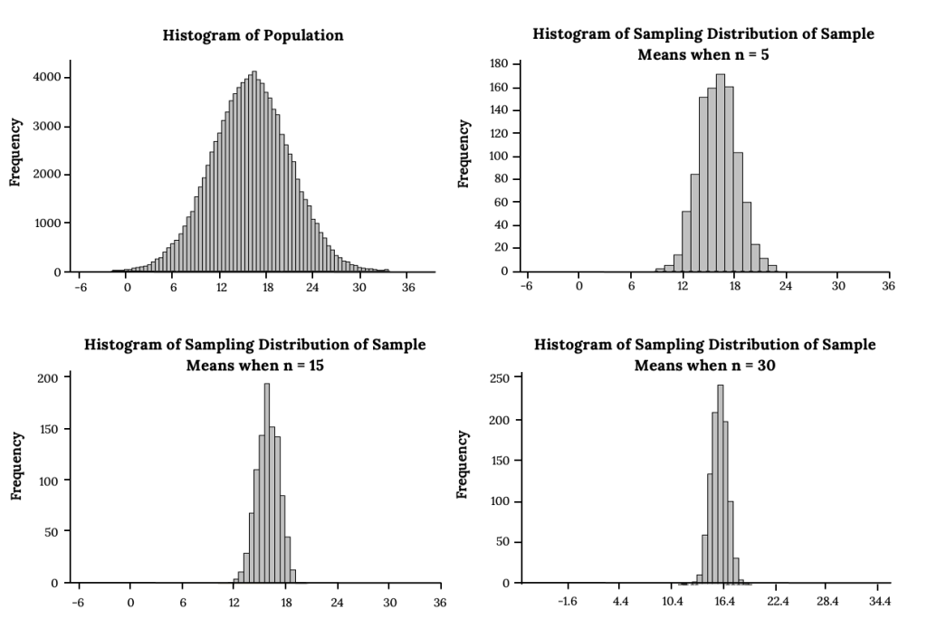
We can develop a better understanding about what the Central Limit Theorem is telling us by using simulation techniques to generate samples from normally distributed populations and from non-normal populations. By simulating the sampling distribution, we develop additional insight into how sample statistics behave. Consider Figure 3 and notice that the histogram of the population shows it is normally distributed. We know from the Central Limit Theorem, that we can take samples of any size and expect the sampling distribution of $\bar{X}$ to also be normally distributed with mean $\mu$ and standard error $\frac{\sigma}{\sqrt{n}}$ . Three sampling distributions are presented, with the sample size, n = 5, 15, and 30, respectively. Notice each histogram showing the sampling distribution of the sample mean is normally distributed and it is easy to see that the standard errors decrease as the sample size increases. This is a nice visual clarification of the meaning of the standard error formula: $\frac{\sigma}{\sqrt{n}}$ . The larger the sample size, the smaller the standard error, and the less uncertainty there is in the distribution of the sample means.

Four distributions as described in the text — Figure 3: Sampling Distributions of the Sample Mean

Now let’s use a simulation to generate sampling distributions of the sample mean when we start with a very non-normally distributed population.

Example 2: Non-Normal Population and the Sampling Distribution of $\bar{X}$

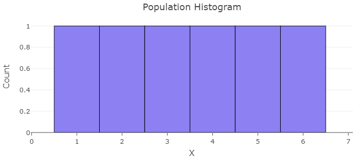
Consider an experiment in which a single six-sided fair die is rolled. The random variable X can take on each of the values 1, 2, 3, 4, 5, and 6 with equal probability, so the population is uniform. Calculate the mean and standard deviation of the population and generate a histogram. Then simulate the sampling distributions using a statistical program for samples of size n = 5, 15, and 30. Summarize your observations as they relate to sampling distribution shape, mean, and standard error compared to the population.

Solutions:

A statistical program created the population histogram of the random variable, X. It shows a uniform distribution with $\mu$ = 3.5 and $\sigma$ = 1.87.

Histogram of the random variable as described in the text with a uniform distribution. — Figure 4: Uniform Distribution of the Population

In order to create the sampling distributions, generate 1000 samples each of size n = 5, 15, and 30 and create the sampling distribution.

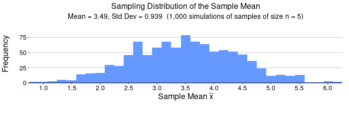
Sampling distribution of the sample mean for n = 5.

For n = 5, we expect $\bar{X}\sim N\bigg(\mu, \frac{\sigma}{\sqrt{5}}\bigg)$ , that is, we expect $\bar{X}\sim N(3.5, 0.836)$ . Notice the simulation gave $\mu_{\bar{X}}$ = 3.49 and $\sigma_{\bar{X}}$ = 0.939. The mean and standard error are both roughly what we expect from the Central Limit Theorem but this is a very small sample size.

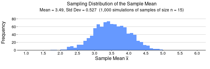
Sampling distribution of the sample mean for n = 15.

For n = 15, we expect $\bar{X}\sim N\bigg(\mu, \frac{\sigma}{\sqrt{15}}\bigg)$ , that is, we expect $\bar{X}\sim N(3.5, 0.836)$ . Notice the simulation gave $\mu_{\bar{X}}$ = 3.49 and $\sigma_{\bar{X}}$ = 0.527. The mean and standard error are both roughly what we expect from the Central Limit Theorem but this is still a small sample size.

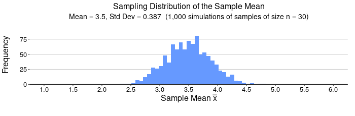
Sampling distribution of the sample mean n = 30

For n = 30, we expect $\bar{X}\sim N\bigg(\mu, \frac{\sigma}{\sqrt{30}}\bigg)$ , that is, we expect $\bar{X}\sim N(3.5, 0.341)$ . Notice the simulation gave $\mu_{\bar{X}}$ = 3.5 and $\sigma_{\bar{X}}$ = 0.387. The mean and standard error are both much closer to what we expect from the Central Limit Theorem.

Notice the striking results! The population was the uniform distribution. While a uniform distribution is symmetric, it is far from normally distributed. Based on the Central Limit Theorem, we would expect to see an approximately normal distribution for the sampling distribution of the sample mean when we reach a sample size of n = 30 but notice how symmetric and somewhat bell-shaped the sampling distributions are for n = 5 and n = 15. If our samples are drawn from nearly symmetric distributions, we can assume the sampling distribution is approximately normal even for small sample sizes. Let’s take a look at the mean and standard errors of the sampling distributions.

Example 3 – Battery Lifetimes

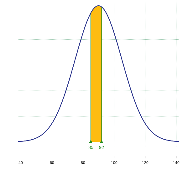
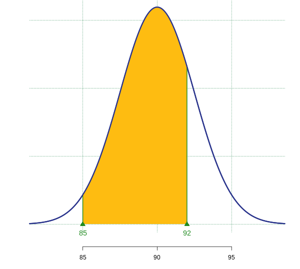
A battery manufacturer claims that under a certain load, a battery has a mean lifetime of 90 hours with a standard deviation of 15 hours. Battery lifetimes are normally distributed. Bulk packages are filled with a random assortment of 36 batteries and are sold in stores.

Find the probability that a single battery will have a lifetime between 85 and 92 hours.
Find the probability that in the package of 36 batteries, the mean lifetime will be between 85 and 92 hours.

Solutions:

The population of batteries is normally distributed, so the random variable X = battery lifetime under a certain load, and $X \sim N(90, 15)$ . When finding probabilities related to a normal distribution, you can find the probabilities directly with a statistical package or you can standardize the normal distribution and find probabilities related to the standard normal distribution. In this case $P(85 < X < 92) = 0.1836.$ A single battery will last between 85 hours and 92 hours approximately 18.36% of the time.
Notice the question has shifted to a probability related to the sample mean. We know from the Central Limit Theorem, that the sample mean is distributed normally, with a mean identical to the population mean of 90 and the standard error calculated as $\frac{\sigma}{\sqrt{36}} = \frac{15}{6} = 2.5$ . In order to calculate the probability, we must use the sampling distribution of the sample mean: $\bar{x} \sim N(90, 2.5)$ . In this case $P(85 < \bar{X} < 92) = 0.7654.$ The mean lifetime of a package of 36 batteries will last between 85 hours and 92 hours approximately 76.54% of the time.

Notice how critical it is for us to always first determine the distribution of the random variable before finding probabilities! A population can have any distribution but the sample mean will have a normal distribution, when the conditions for the Central Limit Theorem are met. This is very powerful!

Videos

YouTube Sampling Distribution of the Sample Mean

Sources

Figure 3: Kindred Grey via Virginia Tech (2021). “Sampling Distributions of the Sample Mean from a Normal Population.” CC BY-SA 4.0. Retrieved from https://commons.wikimedia.org/wiki/File:Sampling_Distributions_of_the_Sample_Mean_from_a_Normal_Population.png

License

Icon for the Creative Commons Attribution 4.0 International License

Introduction to Statistics for Engineers Copyright © by Vikki Maurer & Jeff Crabill & Linn-Benton Community College is licensed under a Creative Commons Attribution 4.0 International License, except where otherwise noted.

Feedback/Errata

Comments are closed.