
7.4 Using the Central Limit Theorem
Learning When to Use the Central Limit Theorem
It is important for you to identify when to use the Central Limit Theorem. The theorem establishes a probability structure for the variable  and thus allows us to compute probabilities of outcomes involving the sample mean.
The following contrast is important to understand. Consider the difference between the following questions:
- What is the probability of kicking one ball more than 100 feet?
- What is the probability of kicking 10 balls more than 100 feet on average?
These two questions differ in a significant way. The first asks a question about the random variable X , which represents the distance one ball is kicked, while the second question asks about the sample mean,  , which is a completely different random variable. Both behave according to different probability structures. Their probabilities will not be the same! Now that we have established the Central Limit Theorem, we have to take care to understand what probability distribution guides our random variable.
Central Limit Theorem Examples
For each of the examples in this section, be sure to pay close attention to the questions asked, which typically have subtle differences. Always know what random variable you are considering and how it is distributed, so you can work with it.
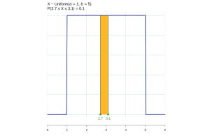
Example 1: Random Variable with Uniform Distribution
A study involving stress is conducted among the students on a college campus. Based on previous work with stress scores, it is known that stress scores follow a uniform distribution, with the lowest stress score equal to one and the highest equal to five. Using a sample of 75 students, find the following:
- Find the probability that a randomly selected student scores between 2.7 and 3.1.
- Find the probability that a randomly selected group of 75 students has a mean score between 2.7 and 3.1.
Solution:
(1)
It is critical that we identify what random variable is being discussed. Here the question is about a single randomly selected student. The random variable  = stress score and the question is asking about how likely it is for a randomly selected score to be between 2.7 and 3.1. We are asked to find
  , where
  . So we can compute this value as an area or by using technology.
  . A randomly selected student will have a score between 2.7 and 3.1 with probability 0.1, or about 10% of students will have this range of scores.
(2)
Notice the change in wording for this question. We are now being asked about a probability related to the sample mean, which is also a random variable and behaves according to the Central Limit Theorem. The random variable has a uniform distribution, but because the sample size is large enough, the sample mean has a normal distribution.
We are asked to find  , where
 .
.
Since  , we know
  .
.
For , we know from our previous study of the uniform distribution that  . Likewise,
  and
and  .
.
Thus,  and we can compute this probability as an area. We find
  . See Figure 2.
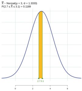
The probability that a randomly selected group of 75 students has a mean score between 2.7 and 3.1 is approximately 0.12, which is greater than the probability for an individual student.
Key Takeaway from the Example Above
They key takeaway from the example above is to understand the difference between  and . The first denotes the chance that ONE observation would fall between 2.7 and 3.1. In contrast, the second denotes the chance that the MEAN of a sample (of size n) would fall between 2.7 and 3.1.
Now look for the same contrast in the next example.
Example 2: Random Variable with Exponential Distribution
A market research analyst for a cell phone company conducts a study of their customers who exceed the time allowance included on their basic cell phone contract. The analyst finds that for those people who exceed the time included in their basic contract, the excess time used follows an exponential distribution with a mean of 22 minutes. Let the random variable = the excess time used by one INDIVIDUAL cell phone customer who exceeds his contracted time allowance. Consider a random sample of 80 customers who exceed the time allowance included in their basic cell phone contract.
- Find the probability that the mean excess time used by the 80 customers in the sample is longer than 20 minutes and draw the graph.
- Suppose that one customer who exceeds the time limit for his cell phone contract is randomly selected. Find the probability that this individual customer’s excess time is longer than 20 minutes.
- Explain why the probabilities in parts 1 and 2 are different.
- Find the 95th percentile for the sample mean excess time for samples of 80 customers who exceed their basic contract time allowances.
Solution: Let’s get organized and make sure we clearly state the distributions of and of . We know refers to the excess time used by one INDIVIDUAL cell phone customer who exceeds his contracted time allowance and refers to the mean excess time used by a sample of 80 customers who exceed their contracted time allowance. From our previous work with the exponential distribution, we know that the mean and standard deviation are the same, so μ = 22 and σ = 22. We also know  , so the parameter
  .
.
 .
.
 by the Central Limit Theorem.
- Find:

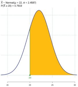
Figure 3: Normal Distribution of Sample Mean - Find
 . Remember to use the exponential distribution for an individual:
  .
. 
- The probabilities are not equal because we use different distributions to calculate the probability for individuals and for means. When asked to find the probability of an individual value, we use the exponential distribution. When asked to find the probability for a mean, we use the distribution of the mean.
- Let
 the 95th percentile. Find
  where
where  . Using a statistical program, we find
  . A vertical line extends from to the curve. The area under the curve to the left of is shaded. The shaded area shows that
  . The 95th percentile for the sample mean excess time used is about 26.0 minutes for random samples of 80 customers who exceed their contractual allowed time. Ninety five percent of such samples would have means under 26 minutes; only five percent of such samples would have means above 26 minutes.
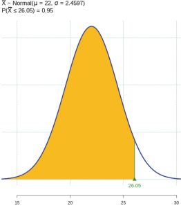
Figure 4: 95th Percentile
Example 3 – Blood Pressure
Based on data from the National Health Survey, women between the ages of 18 and 24 have a systolic blood pressure (in mm Hg) of 114.8 with a standard deviation of 13.1. Systolic blood pressure for women between the ages of 18 to 24 follow a normal distribution.
- If one woman from this population is randomly selected, find the probability that her systolic blood pressure is greater than 120.
- If 40 women from this population are randomly selected, find the probability that their mean systolic blood pressure is greater than 120.
- If the sample were four women between the ages of 18 to 24, and we did not know the original distribution, could the central limit theorem be used?
Solutions:
- The random variable represents the systolic blood pressure for a woman between the ages of 18 and 24.
 . So,
. So,  There is about a 35%, that the randomly selected woman will have a systolic blood pressure greater than 120.
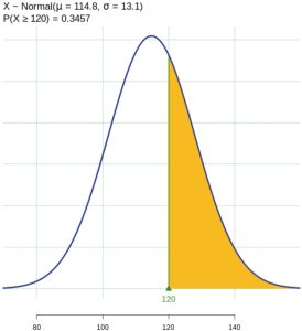
Figure 5: Normal Distribution for Random Variable X - The random variable represents the mean systolic blood pressure of a sample of 40 women.
 . So,
. So,  . There is only a 0.6% chance that the average systolic blood pressure for the randomly selected group is greater than 120.
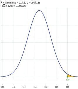
Figure 6: Normal Distribution of Sample Mean - The Central Limit Theorem cannot be used for a sample size of four when we do not know the original distribution. The sample size would be too small.
Example 4 – Male Heights
A new airplane is being designed and all dimensions such as door height, seat width, etc, must consider human physical dimensions. According to a Vital and Health Statistics report, the mean height of males, age 20 and over in United States, is 69 inches, with a standard deviation (interpreted from the report) of 2.9 inches. Because men have a greater average height, this question focuses on males and heights are normally distributed.
- What doorway height would allow 95% of men to enter the aircraft without bending?
- A flight contains 115 men age 20 and over. What doorway height satisfies the condition that there is a 0.95 probability that this doorway height is greater than the mean of the height of 115 men?
- For engineers designing the 757, which result is more relevant: the height from part 1 or part 2? Why?
Solution:
- This question directs us to investigate the random variable representing heights of individual males age 20 and older. We know that
 , so using a statistical package, we find the value
  , such that
  . In this case, a door height of 73.77 inches would allow 95% of males to pass through without bending.
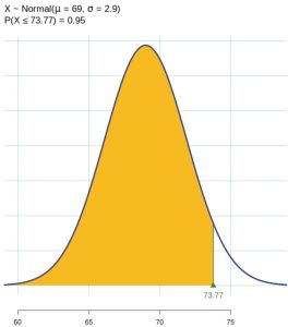
Figure 7: Normal Distribution of Male Heights - Notice how the question has shifted to discussing the mean of 115 men, so we are dealing with the sample mean and have to refer to its sampling distribution. The original population is normal, and we have a large sample size, so we can use the Central Limit Theorem to state
 . Using a statistical package, we find the value , such that , with
  . The doorway height is 69.44 inches.
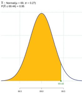
Figure 8: Normal Distribution of Sample Mean - When designing the doorway heights, we need to incorporate as much variability as possible in order to accommodate as many passengers as possible. Therefore, we need to use the result based on part 1.
Historical Note: Normal Approximation to the Binomial
Historically, being able to compute binomial probabilities was a very important applications of the Central Limit Theorem. Binomial probabilities with a small value for  , such as samples up to = 20 were displayed in a table in a reference book for probabilities. These probabilities would go on for pages and pages. To calculate the probabilities with large values of , you had to use the binomial formula, which could be very complicated. Using the normal approximation to the binomial distribution simplified the process.
To compute the normal approximation to the binomial distribution, take a simple random sample from a population. You must meet the conditions for a binomial distribution:
- there are a certain number n of independent trials
- the outcomes of any trial are success or failure
- each trial has the same probability of a success p
Recall that if is the binomial random variable, then  . The shape of the binomial distribution needs to be similar to the shape of the normal distribution under certain circumstances. To ensure this similarity, the quantities
  and
and  must both be greater than five. The approximation is even better if they are both greater than or equal to 10. Then the binomial can be approximated by the normal distribution with mean
  and standard deviation
  . Remember that
  . In order to get the best approximation, add 0.5 to x or subtract 0.5 from x (use x + 0.5 or x – 0.5). Why would we do this? Remember that the binomial distribution is discrete and probabilities are related to areas of rectangles. Since the normal approximation to the binomial would not include the entire rectangle, we add 0.5 to a right-end value and subtract 0.5 from a left-end value to account for the missing probability. The number 0.5 is called the continuity correction factor and is used in the following example.
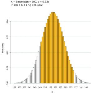
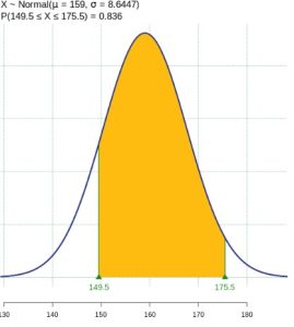
Example 5 – Normal Approximation to the Binomial
Suppose in a local Kindergarten through 12th grade (K – 12) school district, 53 percent of the population favor a charter school for grades K through 5. A simple random sample of 300 is surveyed. Find the probability that between 150 and 175 people favor a charter school. Use the normal approximation to the binomial with and without the continuity correction and use the binomial distribution to calculate the probability directly. Compare the results and provide graphs.
Solution:
The random variable X is defined as the number that favor a charter school for grades K trough 5. Because those surveyed either favor or do not favor a charter school, where = 300 and  = 0.53. Since
  and
and  , use the normal approximation to the binomial. The formulas for the mean and standard deviation are and . The mean is 159 and the standard deviation is 8.6447. Using the normal approximate to the binomial,
  .
.
To incorporate the continuity correction we find  . See Figure 9. Note, without the continuity correction
  . Using the binomial distribution we find
  . See Figure 10. Notice that using the continuity correction provides a much more accurate result.
Sources
“National Health and Nutrition Examination Survey.” Center for Disease Control and Prevention. Available online at http://www.cdc.gov/nchs/nhanes.htm (accessed May 17, 2013).
Vital and Health Statistics, Series 3, Number 46, Table 12. Available online at https://www.cdc.gov/nchs/data/series/sr_03/sr03-046-508.pdf (accessed 7/5/2024).

Feedback/Errata