
8.2 Confidence Interval for the Mean – Large Sample
Confidence Intervals for a Population Mean – Large Sample Size
Interval estimates are often desirable because the estimate of the mean varies from sample to sample. Instead of a single estimate for the mean, a confidence interval generates a lower and upper limit for the mean. The interval estimate gives an indication of how much uncertainty there is in our estimate of the true mean. The narrower the interval, the more precise is our estimate, but as we will see, there is a tradeoff between precision and confidence.
In this section, we will focus on the general construction of a confidence interval for  assuming that we have prior knowledge of the population standard deviation or a large sample size. In practice, in engineering and the sciences, certain types of populations have been worked with so often that the variability is known, so we can use an assumed value for the population standard deviation. For this situation, since the requirements of the Central Limit Theorem are satisfied, and we are working with the the sample mean, we can build confidence intervals based on the normal distribution.

If we do not have prior knowledge of the population standard deviation, and we use the sample standard deviation,  , to estimate of the population standard deviation,
  , then the sample mean may be only approximately normally distributed. For a large sample size, we can choose to use the approximately normal distribution, and you will see this done in practice. However, technically when the sample standard deviation is used in place of the population standard deviation, and the population sampled from is normal, the sample mean behaves according to a new distribution, called the Student’s t distribution, which we will discuss soon.
For now, in this section, we will focus on the form of the confidence interval, assuming prior knowledge of the population standard deviation or assuming a large sample size and an estimated population standard deviation, knowing the underlying distribution is only approximately normal.
Anatomy of a Confidence Interval
Before we proceed to the computation of a confidence interval, study the general anatomy of the confidence interval. Every confidence interval for means will take the the following form, if is known (or can be assumed), and if is estimated and the sample size is large.
Confidence Interval for the Mean
Point Estimate  Margin of Error
Point Estimate (Critical Value)(Standard Error)
 (Critical Value)
-
- The point estimate of the parameter of interest is the calculated statistic, in this case,
 .
. - The critical value is determined from the confidence level.
- The standard error is the standard deviation of the statistic, in this case,
 .
.
- The point estimate of the parameter of interest is the calculated statistic, in this case,
Confidence Level
Confidence intervals are constructed at a specified confidence level, such as 95%, which is selected by the user. This means that if the same population is sampled on numerous occasions and confidence interval estimates are made on each sample, the resulting intervals would contain the true population parameter in approximately 95% of the cases. A confidence stated at a  level can be thought of as the inverse of a significance level,
  .
.
Compute the Critical Value
The critical value is the part of the confidence interval that is calculated from the confidence level. Because the underlying distribution is the normal distribution, and every normal distribution has the same probability structure, we will get critical values from the standard normal distribution. When we use a standard normal distribution to construct the confidence interval, we need to find the z-value that puts an area equal to the confidence level in the middle of the standard normal distribution.
The confidence level is the area in the middle of the standard normal distribution, so if confidence level = 1 – α, then α is the area that is split equally between the two tails. Each of the tails contains an area equal to  . The z-score, critical value, that has an area to the right of is denoted by
  .
.
Example 1 – 95% Confidence Interval Critical Value
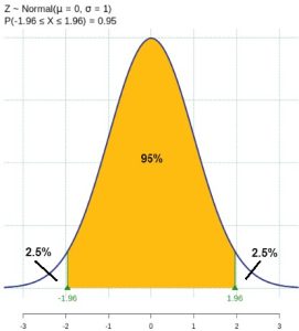
For a 95% confidence interval, calculate and then find the critical value, that is, find the z-value for which 95% of the area under the standard normal curve is centered between +z and -z.
Solution:
The stated confidence level is 95%, so calculate .
0.95 = 1 – , so = 0.05
For a 95% confidence interval, 5% of the area would be in tails of the distribution, with 2.5% in each tail. Using a statistical program, we find the standard normal distribution traps 95% of the centered area between the the z-values z = -1.96 and z = 1.96.
The critical value is 1.96 for a 95% confidence interval.
We would write = 1.96
In Example 1, we found the critical value for a 95% confidence interval, but we could create confidence intervals to any desired level of confidence. In Table 1, for various confidence levels, the corresponding critical values have been determined. You should use a statistical program and verify these values.
| Confidence Level | |
 |
|
 |
| 68% | 0.32 | 0.16 | 1 |  |
| 90% | 0.10 | 0.05 | 1.645 |  |
| 95% | 0.05 | 0.025 | 1.96 |  |
| 99% | 0.01 | 0.005 | 2.576 |  |
| 99.7% | 0.003 | 0.0015 | 2.97 |  |
It should be noted that as the confidence level increases, the critical values get larger. Notice the critical value for a 99% confidence interval is larger than for a 95%, 90%, or a 68% confidence interval. As the confidence level increases, the wider the interval becomes. We can get narrower confidence intervals by decreasing the confidence level but there is a tradeoff between confidence interval width and confidence level.
Writing an Interpretation of a Confidence Interval
The interpretation should clearly state the confidence level, explain what population parameter is being estimated, and state the confidence interval. “We estimate with ___% confidence that the true population mean (include the context of the problem) is between ___ and ___ (include appropriate units).”
Why “Confidence” Rather than “Likely” or “Probability”
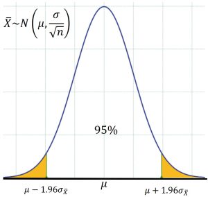
Always keep in mind that when we take a sample from a population to get the sample mean, we obtain just one sample out of possibly an infinite number of possible samples from the sampling distribution of the sample mean.
When we build a confidence interval, such as a 95% confidence interval, we use the known structure of the normal distribution to create a range of values, so that about 95% of the possible sample means exist in that interval. See Figure 2.
If our sample yields one of the sample means in the middle 95% of the distribution, then the true mean will be within the confidence bounds, however, it is possible to get a sample mean that falls into the 5% area of the tails, causing the confidence interval to miss the population parameter entirely. See Figure 3 in which one sample mean came from the middle 95% of the distribution and the confidence interval created contains the true population mean. A second sample mean, although unlikely, came from one of the tails of the distribution, so the resulting confidence interval will not contain the population mean. Imagine taking many samples, obtaining many sample means, and calculating many confidence intervals. In the long run, we would expect 95% of the confidence intervals to contain the true mean. In reality, we create just one confidence interval, so our explanation must reflect the fact that we have confidence in the process.
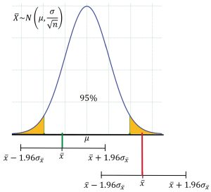
So we state that we have “confidence” in the method we use to create the confidence interval. We know that if we were to create many confidence intervals by taking many samples, then in the long run, 95% of them would contain the true population parameter, and we can specify any level of confidence we want when we build a confidence interval.
Example 2 – Specific Absorption Rate for Cell Phones
The Specific Absorption Rate (SAR) for a cell phone measures the amount of radio frequency (RF) energy absorbed by the user’s body when using the handset. Every cell phone emits RF energy. Different phone models have different SAR measures. To receive certification from the Federal Communications Commission (FCC) for sale in the United States, the SAR level for a cell phone must be no more than 1.6 watts per kilogram. This table shows the highest SAR level for a random selection of cell phone models as measured by the FCC.
| Phone Model | SAR | Phone Model | SAR | Phone Model | SAR |
|---|---|---|---|---|---|
| Apple iPhone 4S | 1.11 | LG Ally | 1.36 | Pantech Laser | 0.74 |
| BlackBerry Pearl 8120 | 1.48 | LG AX275 | 1.34 | Samsung Character | 0.5 |
| BlackBerry Tour 9630 | 1.43 | LG Cosmos | 1.18 | Samsung Epic 4G Touch | 0.4 |
| Cricket TXTM8 | 1.3 | LG CU515 | 1.3 | Samsung M240 | 0.867 |
| HP/Palm Centro | 1.09 | LG Trax CU575 | 1.26 | Samsung Messager III SCH-R750 | 0.68 |
| HTC One V | 0.455 | Motorola Q9h | 1.29 | Samsung Nexus S | 0.51 |
| HTC Touch Pro 2 | 1.41 | Motorola Razr2 V8 | 0.36 | Samsung SGH-A227 | 1.13 |
| Huawei M835 Ideos | 0.82 | Motorola Razr2 V9 | 0.52 | SGH-a107 GoPhone | 0.3 |
| Kyocera DuraPlus | 0.78 | Motorola V195s | 1.6 | Sony W350a | 1.48 |
| Kyocera K127 Marbl | 1.25 | Nokia 1680 | 1.39 | T-Mobile Concord | 1.38 |
Find a 98% confidence interval for the true (population) mean of the Specific Absorption Rates (SARs) for cell phones. Assume that the population standard deviation has been previously estimated as σ = 0.337.
Solution:
To find the confidence interval, start by finding the point estimate, which is the sample mean, = 1.024.
Next, find the standard error for the sample mean, 
Because we are creating a 98% confidence interval,  , so the significance level is 0.02. The critical value which places
  in each tail of the standard normal distribution is needed.

Find  having the property that the area under the standard normal density curve to the right of is 0.01 and the area to the left is 0.99. Using a statistical program, we find
  .
.
To find the 98% confidence interval, find


We estimate with 98% confidence that the true SAR mean for the population of cell phones in the United States is between 0.881 and 1.167 watts per kilogram.
Effect of Changing the Confidence Level or the Sample Size
Inspecting the formula for a generic confidence interval will lead to the following conclusions:
- Increasing the confidence level increases the margin of error, making the confidence interval wider.
- Decreasing the confidence level decreases the margin of error, making the confidence interval narrower.
- Increasing the sample size causes the margin of error to decrease, making the confidence interval narrower.
- Decreasing the sample size causes the margin of error to increase, making the confidence interval wider.
Example 3 – Change the Sample Size or the Confidence Level
- A 95% confidence interval for a population mean is calculated from a sample size of 400. A second 95% confidence interval is calculated from a sample drawn from the same population with a sample size of 100. Compare the widths for the resulting confidence intervals.
- A 95% confidence interval for a population mean is calculated from a sample size of 100. A second 68% confidence interval is calculated from a sample drawn from the same population with a sample size of 100. Compare the widths of the resulting confidence intervals.
Solution:
- A 95% confidence interval for the population mean is calculated as
 . Notice we do not have any data to use so we will analyze these intervals symbolically. We do know = 0.05, so the critical value is 1.96.
Sample Size of 400: gives
gives  .
.
Sample Size of 100: gives
gives  .
.
Notice how changing the sample size affects the width of the interval. A sample size of 100 produces an interval twice as wide. The interval produced from the sample size of 400 will be half as wide. The greater the sample size, the better the estimates of the population parameters, so the narrower the intervals. - A confidence interval for the population mean is calculated as
 . Notice we do not have any data to use so we will analyze these intervals symbolically.
For a 95% confidence interval, with n = 100, we do know = 0.05, so the critical value is 1.96.
For a 68% confidence interval, with n = 100, we do know = 0.16, so the critical value is 1.
95% Confidence Interval: gives .
68% Confidence Interval: gives
gives  .
.
For these two confidence intervals, the only difference is the critical value. The 95% confidence has a critical value that is almost twice the size of the critical value for the 68% confidence interval. The resulting interval will be twice as wide. There is a tradeoff when the confidence level is increased. The interval becomes wider with more confidence. With less confidence, the confidence interval becomes narrower.
Calculating the Sample Size n
If researchers desire a specific margin of error, then they can use the error bound formula to calculate the required sample size. Simple algebra gives the formula.
The error bound formula for a population mean when the population standard deviation is known is  . Use a value of
  appropriate for your desired confidence level.
Some elementary algebra yields  , thus giving us a useful formula for sample size needed for our specific error bound.
Example
The population standard deviation for the age of Foothill College students is 15 years. If we want to be 95% confident that the sample mean age is within two years of the true population mean age of Foothill College students, how many randomly selected Foothill College students must be surveyed?
- From the problem, we know that σ = 15 and e = 2.
- z = zcv = 1.96, because the confidence level is 95%.
- using the sample size equation.
- Use n = 217: Always round the answer UP to the next higher integer to ensure that the sample size is large enough.
Therefore, 217 Foothill College students should be surveyed in order to be 95% confident that we are within two years of the true population mean age of Foothill College students.
Videos
YouTube Video Confidence Interval for the Mean
Sources
La, Lynn, Kent German. “Cell Phone Radiation Levels.” c|net part of CBX Interactive Inc. Available online at http://reviews.cnet.com/cell-phone-radiation-levels/ (accessed July 2, 2013).

Feedback/Errata