
8.4 Small Sample Confidence Intervals and the Student’s t-Distribution
We have discussed the sampling distribution of the sample mean when the population standard deviation,  , is known. However, in practice, we rarely know the population standard deviation. In the past, when the sample size was large, this did not present a problem to statisticians. They used the sample standard deviation
  as an estimate for and proceeded as before to calculate a confidence interval with close enough results. However, statisticians ran into problems when the sample size was small. A small sample size caused inaccuracies in the confidence interval.
William S. Gosset (1876–1937) of the Guinness brewery in Dublin, Ireland ran into this problem. His experiments with hops and barley produced very few samples. Just replacing with did not produce accurate results when he tried to calculate a confidence interval. He realized that he could not use a normal distribution for the sampling distribution. This is because is a more reliable estimate of as samples get bigger. He found that the actual distribution of the sample mean depends on the sample size. This problem led him to “discover” what is called the Student’s t-distribution. The name comes from the fact that Gosset wrote under the pen name “Student.”
Up until the mid-1970s, some statisticians used the normal distribution approximation for large sample sizes and only used the Student’s t-distribution only for sample sizes of at most 30. With graphing calculators and computers, the practice now is to use the Student’s t-distribution whenever the sample standard deviation is used as an estimate for the population standard deviation, .
Student’s t-Distribution
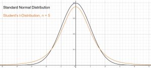
The Student’s t-distribution is similar to the standard normal distribution in that they are both symmetric about a mean of zero. Both of these distributions are bell shaped, but the Student’s t-distribution allows for more variability. Remember, we are dealing with the situation where we have a smaller sample and we are using the sample standard deviation to estimate the population standard deviation, so there are two sources of variation, the sample mean and the sample standard deviation. The smaller the sample, the more the sample variance will fluctuate from sample to sample, so we will see that the Student’s t-distribution has a different probability distribution depending on the sample size. As the sample size grows, the sample variance becomes a better approximator of the population variance, so as  , the two distributions will become indentical.
If you draw a simple random sample of size  from a population that has an approximately a normal distribution with mean
  and unknown population standard deviation, , and calculate the following t-score,

then the t-score has a Student’s t-distribution, with  degrees of freedom. Keep in mind that for each sample size , there is a different Student’s t-distribution. The smaller the sample size, the more variation that needs to be accounted for, so each sample size requires the use of a different version of the Student’s t-distribution. See Figure 1 for a comparison of the standard normal distribution with a Student’s t-distribution for a sample size of five, so four degrees of freedom. Notice that there is more area in the tails of the distribution to account for the increased variation.
The degrees of freedom, abbreviated as d.f. and noted as , come from the calculation of the sample standard deviation . Because the sum of the deviations of each value from the mean is zero, we can find the last deviation once we know the other deviations. The other deviations can change or vary freely. For us, we need to remember that as the sample size gets smaller, sample variances fluctuate more, so the Student’s t-distribution accounts for that increased variation by forcing more area into the tails of the distribution.
Properties of the Student’s t-Distribution
- The graph for the Student’s t-distribution is similar to the standard normal curve in that they are both bell shaped.
- The mean for the Student’s t-distribution is zero and the distribution is symmetric about zero.
- The Student’s t-distribution has more probability in its tails than the standard normal distribution because the spread of the t-distribution is greater than the spread of the standard normal. So the graph of the Student’s t-distribution will be thicker in the tails and shorter in the center than the graph of the standard normal distribution.
- The exact shape of the Student’s t-distribution depends on the size of the sample, , and for each sample size there are degrees of freedom. As the degrees of freedom increases, the graph of Student’s t-distribution becomes more like the graph of the standard normal distribution.
- The underlying population of individual observations is assumed to be normally distributed with unknown population mean μ and unknown population standard deviation σ. The size of the underlying population is generally not relevant unless it is very small. If it is bell shaped (normal) then the assumption is met and does not need discussion. Random sampling is assumed, but that is a completely separate assumption from normality.
Confidence Interval for Population Mean, Small Sample
A random sample of size is taken from a normal (or approximately normal) population with unknown .
The 100(1 –  )% Confidence Interval for is given as
Sample Mean  (Critical Value)(Standard Error)

Where  is the
  -value with degrees of freedom, leaving an area of
  to the right.
Assumptions
When the sample comes from a normal distribution, or an approximately normal distribution, the Student’s t-distribution is appropriate. We do not always know the distribution of the population. If we use a distribution without verifying the assumptions have been met, then we run the risk of reporting information that is misleading. Sometimes there is enough past history with a population, so that it’s underlying distribution can be assumed. However, if the population distribution is completely unknown, then it is important to check into the normality assumption before moving forward with the Student’s t-distribution.
A sad fact with small sample sizes is that if we have to investigate the sample to gain insight into the distribution of the population, small samples make it hard to detect departures from normality. What we can do is construct a box plot or a dot plot to see if there is strong asymmetry or if outliers exist. Remember that normal distributions rarely contain outliers, so if you see outliers showing up in the sample, it may indicate the underlying population is not normally distributed. A normal probability plot of the sample data can also be used to investigate the distribution of the population.
Example 1 – Compressive Strength of Concrete
A measure of performance and strength of a concrete mixture is its compressive strength, in megapascals (MPa). Compressive strength is the ability of a concrete material to carry the load on its surface without crack or deflection. The strength of concrete increases with age. On day 28, concrete should have 99% of its compressive strength. Testing concrete on day 7, when concrete is expected to have 65% of its strength, can help detect potential problems with quality. A random sample of ten cylindrical specimens of M40 grade concrete were tested on day 7 with the following measurements: 26.5, 26.0, 27.0, 24.3, 28.1, 27.9, 29.5, 27.2, 23.5, 25.0.
- Determine if it is appropriate to use a Student’s t-distribution to construct a confidence interval for the mean concrete strength.
- Find a 95% confidence interval for the mean compressive strength.
Solutions:
-
We do not have information about the population from which this sample is drawn and the sample size is small, so it is important to examine the sample to see if there is any departure from normality. By examining the box plot in Figure 2, it shows the sample is symmetric and there are no outliers, so we will assume the data come from a normal distribution.
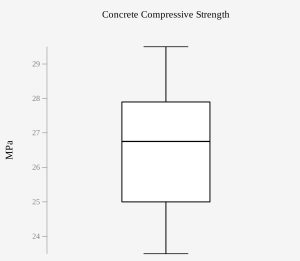
Figure 2: Box Plot of Concrete Strengths -
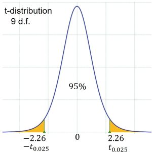
Figure 3: t-distribution with 9 d.f. For this sample, the sample mean,
 = 26.5 MPa and the standard deviation, = 1.844 MPa. The sample size is 10, so use the Student’s t-distribution with = 9 degrees of freedom. The critical value from the t-distribution with 9 degrees of freedom is
  as shown in Figure 3.
The 95% confidence interval is constructed as


26.5 1.318
(25.18, 27.82)The 95% confidence interval for the mean concrete strength is (25.18 MPa, 27.82 MPa).
Example 2 – Industrial Pollution
The Human Toxome Project (HTP) is working to understand the scope of industrial pollution in the human body. Industrial chemicals may enter the body through pollution or as ingredients in consumer products. In October 2008, the scientists at HTP tested cord blood samples for 20 newborn infants in the United States. The cord blood of the “In utero/newborn” group was tested for 430 industrial compounds, pollutants, and other chemicals, including chemicals linked to brain and nervous system toxicity, immune system toxicity, and reproductive toxicity, and fertility problems. There are health concerns about the effects of some chemicals on the brain and nervous system. This table shows how many of the targeted chemicals were found in each infant’s cord blood.
| 79 | 145 | 147 | 160 | 116 | 100 | 159 | 151 | 156 | 126 |
| 137 | 83 | 156 | 94 | 121 | 144 | 123 | 114 | 139 | 99 |
There has been extensive study with this population and it can be assumed to be normally distributed. Use this sample data to construct a 90% confidence interval for the mean number of targeted industrial chemicals to be found in an in infant’s blood.
Solution:
From the sample, the sample mean is calculated as = 127.45 with a sample standard deviation of = 25.97. The sample size is 20, so we will use the Student’s t-distribution with 19 d.f.. To create the 90% confidence interval, we find the t-critical value that places 5% of the area in each tail. Using a statistical program, we find  = 1.73. The 90% confidence interval is constructed as
.


127.45 10.05
(117.4, 137.5)
It is estimated with 90% confidence that the mean number of targeted industrial chemicals found in an infant’s blood is between 117.4 and 137.5.
Sources
AskCivilEngineer.com. (n.d.). Compressive strength of Concrete – Test, results & procedure. https://askcivilengineer.com/compressive-strength-of-concrete/
“Human Toxome Project: Mapping the Pollution in People.” Environmental Working Group. Available online at http://www.ewg.org/sites/humantoxome/participants/participant-group.php?group=in+utero%2Fnewborn (accessed July 2, 2013).

Feedback/Errata