
9.6 Hypothesis Testing Errors and Power
Although hypothesis testing provides a strong framework for making decisions based on data, as the analyst, you need to understand how and when the process can go wrong. It is important to always keep in mind that the conclusion to a hypothesis test might not be correct! Sometimes when the null hypothesis is true, we will actually reject it. Sometimes when the alternative hypothesis is true, we will fail to reject the null hypothesis. If we know errors can be made, what can we do about them? Can we make the likelihood of making errors small? What about making correct decisions? How can we quantify the probability of rejecting the null hypothesis when it is not true? These are all important considerations we will introduce in this section. However detailed explorations of these ideas will occur in later statistics courses you take.
Decision-Making Errors
When performing a hypothesis test, there are four possible outcomes depending on the actual truth or falseness of the null hypothesis  and the decision to reject or not reject.
- The decision to fail to reject could be the correct decision.
- The decision to fail to reject could be the incorrect decision.
- The decision to reject could be the correct decision.
- The decision to reject could be the incorrect decision.
Type I Error: The decision is to reject when it is actually true is an incorrect decision known as a type I error.
 represents the probability of a type I error.
- P(Type I Error) represents the probability of rejecting the null hypothesis when the null hypothesis is actually true
- The probability of a type I error is also called the level of significance.
Type II Error: The decision to fail to reject when it is actually false is an incorrect decision known as a type II error.
 represents the probability of a type II error.
- P(Type II Error) represents the probability of not rejecting the null hypothesis when the null hypothesis is actually false.
 represents the probability of rejecting the null hypothesis when it is actually false.
- In other words, represents the probability of making a correct decision when the null hypothesis is false and is the power of the test.
Hypothesis Testing Decision Options
| is Actually |
|||
|---|---|---|---|
| True | False | ||
| Decision | Fail to reject |
Correct Outcome,  |
Type II error, |
| Reject |
Type I Error, |
Correct Outcome, Power |
|
Example 1 – Toxic Clams and Decision Making Errors
“Red tide” is a bloom of poison-producing algae, produced by a few different species of a class of plankton called dinoflagellates. When the weather and water conditions cause these blooms, shellfish such as clams living in the area develop dangerous levels of a paralysis-inducing toxin. In Massachusetts, the Division of Marine Fisheries (DMF) monitors levels of the toxin in shellfish by regular sampling of shellfish along the coastline. If the mean level of toxin in clams exceeds 800  (micrograms) of toxin per 100 grams of clam meat in any area, clam harvesting is banned there until the bloom is over and levels of toxin in clams subsides. State the null and alternative hypotheses and describe both a Type I and a Type II error in this context. Then explain which error has the greater consequence.
Solutions:
In this scenario, the status quo is to allow clamming and assume algae levels are safe until there is proof otherwise. An appropriate null hypothesis would be : The mean level of toxins is at most 800 . An appropriate alternate hypothesis would be  : The mean level of toxins is greater than 800 .
: 
: 
- Type I error: The DMF rejects the null hypothesis and concludes the toxin levels are too high when, in fact, toxin levels are at a safe level. The DMF bans harvesting, when it is actually safe to harvest. This error will cost those who depend on harvesting and selling clams for income.
- Type II error: The DMF fails to reject the null hypothesis and concludes that toxin levels are within acceptable levels, when in fact toxin levels too high. As a result the DMF continues to allow harvesting of clams. This error can possibly harm humans, as consumers could possibly eat tainted food.
Arguably, the more dangerous error would be to commit a Type II error, because this error involves the availability of tainted clams for consumption.
Errors
It does not make sense to conduct an experiment that has a large probability of leading to an incorrect decision. When action will be taken as the result of rejecting the null hypothesis, we want to have an acceptable probability of making a type I error. Both the probability of making a type I error, , and the probability of making a type II error, , should be as small as possible because they are probabilities of errors, but they are rarely zero.
We choose the probability of committing a type I error by selecting , the significance level, in advance. If the null hypothesis is rejected, then we are either make the right decision or we make a type I error with a known and chosen probability. This allows for a “strong” statement to be made regarding a rejection.
If the null hypothesis is not rejected, we either make the right decision, or we make a type II error, which has an unknown probability. We label this probability as , but as we will see, we cannot reliably calculate it. We cannot make a strong statement, in the case when we fail to reject the null hypothesis. In fact, we normally defer the decision and just say there is not enough evidence to indicate that we should reject the null hypothesis, and so in a sense, make no decision at all. This is the reason that what you really want to know is put in the alternate hypothesis. If a claim is made in the null hypothesis, and that claim is not correct, you would really like to know about it. Reducing the probability of a type II error is of course desirable, but is of secondary importance.
Controlling the Type I Error Rate
The probability of a type I error is also called the significance level, . The significance level is selected and set at some prespecified level such as 5% or 1%, with 5% being the most widely used level. In order to reduce the type I error rate, we have to raise the evidence requirement for rejection of the null hypothesis. We can make the probability of a type I error as small as we want, however, unfortunately as the probability of a type I error decreases, the probability of a type II error increases. This is why a significance level of 5% is often set. It provides a “reasonably” small type I error.
If the type II error is estimated and found to be too big then the experiment should be redesigned, but how do we calculate it? Remember that a type II error is made when the alternate hypothesis is true but we fail to reject the null hypothesis. The core issue with trying to calculate it is there are an infinite number of ways that the alternate hypothesis can be true, and the probability of a type II error depends on knowing the true population parameter, which is precisely the thing we are estimating! While we cannot calculate the exact probability of a type II error in general, we can get a sense of it by trying out some possible values of the parameter under the alternate hypothesis.
Example 2 – Probability of a Type II Error with Toxic Algae
Let’s reconsider the toxic algae hypothesis test from Example 1. Recall that if the mean level of toxin in clams exceeds 800 of toxin per 100 grams of clam meat in any area, clam harvesting is banned there until the bloom is over and levels of toxin in clams subside. A sample of 50 clams will be randomly selected. Let’s set an level of 0.05. Assume the Division of Marine Fisheries has sampled in this region for so many years, that they estimate the population standard deviation to be 25 .
:
:
- Create a graph of the critical region for this hypothesis test to visualize the probability of making a type 1 error.
- Suppose the true mean toxin level is
 = 802 . Use that value to calculate the probability of making a type II error and provide a graph to visualize this probability. What do you notice?
 - Suppose the true mean toxin level is = 812 . Use that value to calculate the probability of making a type II error and provide a graph to visualize this probability. What do you notice?
Solutions:
- We set = 0.05. Under the null hypothesis we assume
 = 800, the sample size is
  = 50, and we know
  = 25. The null hypothesis will be rejected if
  is greater than 1.645 because
  . Solving for the sample mean, the null hypothesis will be rejected if
  . Any statistical program will also allow you to find this value directly using the distribution of the sample mean,
  . This critical region is shaded in Figure 1.
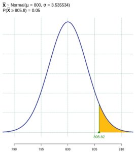
Figure 1: The Critical Region - A type II error is committed if the null hypothesis is false but we fail to reject the null hypothesis, so the sample mean does not fall in the critical region. We are given a true value of the population mean to work with, so find
 for the alternate hypothesis distribution of
  . See Figure 2 in which this probability is shaded and is equal to 0.86. Notice this probability is quite large. Because the true mean of 802 was not very different from the null hypothesis value of 800, this test has a very high probability of making a type II error.
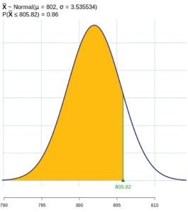
Figure 2: Probability of a Type II Error - A type II error is committed if the null hypothesis is false but we fail to reject the null hypothesis. We are given a true value of the population mean to work with, so find
 for the alternate hypothesis distribution of
  . See Figure 3. Notice this probability is much smaller than what we found in part (2). Because the true mean of 812 was very far from the null hypothesis value of 800, this test has a low probability of making a type II error. The probability of making a type II error is approximately 0.04 in this case.
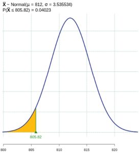
Figure 3: Probability of a Type II Error
Summary of Errors
- There are two types of errors that can be made when conducting a hypothesis test. Rejecting the null hypothesis when it is true is a type I error. Failing to reject the null hypothesis when it is false is a type II error.
- After completing a hypothesis test, we will not know which error was made (if one was made at all) because we will never know the true value of the population parameter on which the hypothesis test is based.
- The size of the critical region can always be reduced, so the size of the type I error can be reduced.
- Reducing the probability of a type I error increases the probability of a type II error, and vice versa.
- The probability of committing a type II error increases greatly and is maximized when the true parameter is close to the null hypothesis value of the parameter.
- The greater the distance between the true value of the parameter and the null hypothesis value, the smaller the probability of a type II error.
- Taking larger samples is a good way to reduce both types of error, simultaneously.
Power
Take another look at Table 1. The decision to reject when it is actually false is a correct decision whose probability is called the Power of the test. When planning a study, we want to know how likely we are to detect an effect we care about. In other words, if there is a real effect (null hypothesis is false), and that effect is large enough that it has practical value, then what is the probability that we detect that effect (reject the null hypothesis)? We can compute the power of a test for different sample sizes or different effect sizes.
Power = , so Power = 1 – P(Type II Error)
Although we will not go into extensive detail, power is an important topic for follow-up consideration after understanding the basics of hypothesis testing. The power of the test is the probability of correctly rejecting the null hypothesis (when the alternative alternative hypothesis is true). We want a hypothesis test to be powerful.
Example 3 – Power
Reconsider the type II error calculations from Example 2. Recall that we could not calculate a value for unless we selected a possible true mean toxin level. For each calculation of in Example 2, calculate the power of the test.
Solutions:
- In the case when the true mean was thought to be = 802, the value of was 0.86. The power of that test would be calculated as = 1 – 0.86 = 0.14. The test has very low power. There is a 14% chance of making a correct decision if the null hypothesis is false.
- In the case when the true mean was thought to be = 812, the value of was 0.04. The power of that test would be calculated as = 1 – 0.04 = 0.96. The test has very high power. There is a 96% chance of making a correct decision if the null hypothesis is false.
A good power analysis is a vital preliminary step to any study as it will inform whether the data you collect are sufficient for being able to conclude your research broadly. Often times in experiment planning, there are two competing considerations:
- We want to collect enough data that we can detect important effects.
- Collecting data can be expensive, and, in experiments involving people, there may be some risk to patients.
You might be interested to know that, often, paired t-tests are more powerful than independent t-tests because the pairing reduces the inherent variability across observations. Additionally, because the median is almost always more variable than the mean, tests based on the mean are more powerful than tests based on the median. That is to say, reducing variability, done in different ways depending on the experimental design and set-up of the analysis, makes a test more powerful in such that the data are more likely to reject the null hypothesis.
Videos
YouTube Video Khan Academy What is a Type I Error
Sources
Red Tide (Paralytic Shellfish Poisoning). (n.d.). Commonwealth of Massachusettes. Retrieved July 18, 2024, from https://www.mass.gov/info-details/red-tide-paralytic-shellfish-poisoning
Hollingsworth, H., & Salter, J. (2024, July 20). Murder conviction overturned for Missouri woman who served 43 years | AP News. AP News. https://apnews.com/article/sandra-hemme-conviction-overturned-56831edcb2aa99b0430c0dbf0408dc5d?utm_source=Email&utm_medium=share

Feedback/Errata