10.3 Inference for Paired Samples

Jeff Crabill; Vikki Maurer

10.3 Inference for Paired Samples

When we conduct a study involving the same participants who have been measured at two points in time, we are working with paired samples. This type of experimental design allows researches to control for confounding variables. Compare this to the situation with two independent samples, in which there are differences between the sampling units that contribute to the variability in the data. By creating a meaningful pairing, other differences that would exist with independent samples are eliminated, so a source of variability has been reduced, and the focus can be on the treatment differences. By eliminating a source of variation, the estimate of the standard deviation will be smaller, increasing the power of the the test. If the treatment is not effective, then the expectation is that the responses from each individual at both points in time would be similar, so the difference would be close to zero.

In the paired sample case, researchers measure the same participants. The measurement for each participant will be taken at two distinct time points. In order to analyze the data, the differences are examined. Consider several scenarios:

Ten vehicles are selected randomly from a particular fleet and each vehicle had emissions measured for highway driving and city driving. The mean of the ten measures of emissions for highway driving is $\mu_1$ and the mean of the ten emission measures for city driving is $\mu_2$ . The mean difference between emissions, $\mu_1 - \mu_2 = \mu_d$ is the target of investigation. There are 10 mean differences to examine and the focus on the investigation is to determine if there is evidence to conclude $\mu_d \neq 0$ .
Thirteen adult females between the ages of 50 and 70 participate in a study to evaluate the effect of diet on blood cholesterol levels. The mean blood cholesterol level is measured for the 13 individuals initially, $\mu_1$ , and then again after three months on a diet, $\mu_2$ . There are 13 mean differences to examine. If diet has no effect, the expectation is that the mean difference, $\mu_1 - \mu_2 = \mu_d$ will be close to zero. If the diet is effective then the expectation is that after the treatment, the blood cholesterol level will be reduced. Thus, researchers will determine if there is evidence to conclude $\mu_d > 0$ .
A maintenance manager will test a new repair method on 9 of the injection molding machines to see if a new repair method increases the expected time between repairs. The mean time between repairs for each of the 9 machines prior to the intervention is $\mu_1$ . After the new repair method is employed, the mean time between repairs for each machine is recorded as $\mu_2$ . If the new repair technique makes no difference in the time between repairs, then the expectation is that mean difference $\mu_1 - \mu_2 = \mu_d$ will be close to zero. The target of the investigation is to see if there is evidence to conclude $\mu_d > 0$ , so the 9 mean differences will be examined.

Paired-Samples Inference

For a matched pair or paired sample inference, the following characteristics and assumptions should be present:

Simple random sampling is used.
There are no outliers.
Two measurements (samples) are drawn from the same pair of individuals or objects.
The variable of interest is measured on a continuous scale.
Differences are calculated from the matched or paired samples.
The differences form the sample that is used for the hypothesis test or confidence interval.
The matched pairs have differences that come from a population of differences that is normal or the sample should be large.

As we have learned, when we use the Student’s t-distribution, the population from which the data comes must be normally distributed. For paired samples, the normality assumption applies to the population of paired differences rather than the raw data. As long as the paired differences do not show significant skewness and the sample size is large enough, the Student’s t-distribution can be used, thanks to the Central Limit Theorem.

In a hypothesis test for matched or paired samples, subjects are matched in pairs and differences are calculated. The differences are the data values under analysis. The population mean for the differences, $\mu_d$ , is then tested using a Student’s-t test for a single population mean with $n$ – 1 degrees of freedom, where $n$ is the number of differences.

Inference for Paired Samples

When performing inference for paired data involving a single population mean difference, $\mu_d$ , the underlying sampling distribution of the sample mean difference, $\bar{x}_d$ is the Student’s t-distribution as long as there was simple random sampling and the population of differences is approximately normally distributed.

Hypothesis Testing

To test a null hypothesis of the form $H_o: \mu_d = \mu_o$ ; $H_o: \mu_d \geq \mu_o$ ; or $H_o: \mu_d \leq \mu_o$ ,

We assume $H_o$ is true, so the null distribution is $\bar{x}_d \sim t_{n-1} \bigg(\mu_o, \frac{s_d}{\sqrt{n}}\bigg)$

The test statistic (t-score) is $\displaystyle{t = \frac{\bar{x}_d - \mu_o}{\frac{s_d}{\sqrt{n}}}}$

Probability associated with the test statistic can be found from the Student’s t-distribution with $n - 1$ degrees of freedom. Equivalently, the p-value can be found using the null distribution directly.

If $H_a: \mu_d \neq \mu_o$ , calculate the p-value as the sum of the areas in the tails cut off by $-t$ and $t$ . $t$

If $H_a: \mu_d < \mu_o$ calculate the p-value as the area to the left of the test statistic, $t$ .

If $H_a: \mu_d > \mu_o$ calculate the p-value as the area to the right of the test statistic, $t$ . $t$

Confidence Interval

The two-tailed hypothesis test is equivalent to finding a $(1 - \alpha)100$ % confidence interval for $\mu_d$ and failing to reject $H_o: \mu_d = \mu_o$ if the test statistic falls inside the confidence interval:

$\displaystyle{\bar{x}_d \pm t_{n-1, \frac{\alpha}{2}}\bigg(\frac{s_d}{\sqrt{n}}\bigg)}$

Example 1 – Pain Reduction Through Hypnotism

A study was conducted to investigate the effectiveness of hypnotism in reducing pain. Results for randomly selected subjects are shown in Table 1. A lower score indicates less pain. For each subject, the pain level is recorded, and then after the treatment, the pain level is recorded again. Assume the differences have a normal distribution. Is there evidence to conclude that average pain levels are lower after treatment with hypnotism? Conduct a hypothesis test at a 5% significance level. Then create the 95% confidence interval for the mean difference in pain after hypnotism and compare the result to the hypothesis test.

Table 1: Pain Levels Before and After Hypnotism
Subject:	A	B	C	D	E	F	G	H
Before	6.6	6.5	9.0	10.3	11.3	8.1	6.3	11.6
After	6.8	2.4	7.4	8.5	8.1	6.1	3.4	2.0

Solution:

Calculate the differences for each of the matched pairs as shown in Table 2. Note that by creating the difference as (Pain Level After Treatment – Pain Level Before Treatment), when the difference is negative, it means the subject showed an improvement, so a decrease in pain.

Table 2: Differences in Matched Pairs
After Treatment	Before Treatment	After – Before = Difference
6.8	6.6	0.2
2.4	6.5	-4.1
7.4	9	-1.6
8.5	10.3	-1.8
8.1	11.3	-3.2
6.1	8.1	-2
3.4	6.3	-2.9
2	11.6	-9.6

In order to test the hypothesis that pain levels are reduced after treatment, the alternate hypothesis will state that the mean difference is less than 0. The null hypothesis is zero or positive, meaning that there is the same or more pain felt after hypnotism.
$H_o: \mu_d \geq 0$
$H_o: \mu_d < 0$
The data for the hypothesis test are the eight differences: {0.2, –4.1, –1.6, –1.8, –3.2, –2, –2.9, –9.6} and we assume the differences come from a normal distribution. We will use a t-test statistic with $n - 1 = 8 - 1 = 7$ degrees of freedom. Without that assumption, we could create a normal probability plot to assess the normality of the differences. The sample mean and sample standard deviation of the differences are $\bar{x}_d = -3.125$ and $s_d = 2.9114$ Verify these values. We begin the hypothesis by assuming the null hypothesis is true, so the sample mean difference is distributed as $\bar{x}_d \sim t_{7}\bigg(0, \frac{2.9114}{\sqrt{8}}\bigg)$ .
The test statistic is $\displaystyle{t = \frac{-3.125 - 0}{\frac{2.9114}{\sqrt{8}}}} = -3.0359$ .
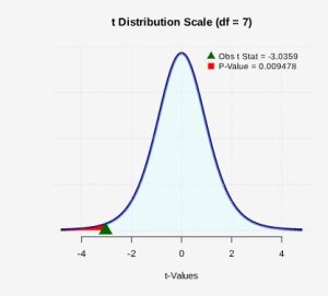
The p-value is the probability of observing a sample mean difference as extreme as we did under the assumption that the null hypothesis is true. A statistical program can show the p-value based on the sampling distribution or on the distribution of the test statistic, both of which are shown in Figure 1.

Figure 1: P-value Visualization

The p-value is the probability $P(t \geq -3.0359) \approx 0.0095$ or approximately 0.95%. Alternatively, and equivalently, the p-value can be calculated directly as $P(\bar{x}_d \geq -3.125) \approx 0.0095$ .
Assuming the null hypothesis is true, the probability we would observe a sample mean difference as extreme as the one we observed is 0.0095. There is less than a 1% chance of observing a sample as least as extreme as we did, which a small probability and less than a 5% level of significance. Because this is highly unlikely, we conclude that we have evidence to reject the null hypothesis. The data supports the claim that the mean pain level after hypnosis is less than before hypnosis.

The 95% confidence interval for the mean difference in pain after hypnotism is calculated as

$\displaystyle{\bar{x}_d \pm t_{n-1, \frac{\alpha}{2}}\bigg(\frac{s_d}{\sqrt{n}}\bigg)}$
$\displaystyle{-3.125\pm t_{7, 0.025}\bigg(\frac{2.9114}{\sqrt{8}}\bigg)}$
$\displaystyle{-3.125\pm 2.365(1.0293)}$
$\displaystyle{-3.125\pm 2.434}$
$(-5.96, -0.69)$

With 95% confidence the mean difference in pain after hypnosis, $\mu_d$ is in the interval (-5.96, -0.69). Note the interval does not include the value 0, so the null hypothesis from the hypothesis test was rejected at a 5% significance level.

License

Icon for the Creative Commons Attribution 4.0 International License

Introduction to Statistics for Engineers Copyright © by Vikki Maurer & Jeff Crabill & Linn-Benton Community College is licensed under a Creative Commons Attribution 4.0 International License, except where otherwise noted.

Feedback/Errata

Comments are closed.