
9.4 Hypothesis T-Test for a Single Mean
In engineering, precise and accurate data analysis is crucial for making informed decisions, optimizing processes, and ensuring safety. When performing a hypothesis test of a single population mean  using a normal distribution z-test, a simple random sample is taken from the population, the population is normally distributed or your sample size is sufficiently large, and the value of the population standard deviation is known. What is often the case is that the population standard deviation is not known, so it must be estimated. Due to the increased variation in the distribution of the sample statistic, the z-test is not an appropriate test, and we switch to the t-test, especially with small sample sizes.
When dealing with small sample sizes, we have noted that the Student’s t-distribution accommodates the increased variability and uncertainty inherent in smaller datasets. In this case, the t-distribution provides a more accurate reflection of the true population parameters, enabling engineers to perform hypothesis testing and construct confidence intervals with greater reliability. This nuanced approach ensures that the conclusions drawn from statistical analyses are robust, even when data is limited. When performing inference on a single population mean
using a Student’s t-distribution, which is called a t-test, there are fundamental assumptions that need to be met in order for the test to be reliably used. The data should be a simple random sample that comes from a population that is approximately normally distributed and the sample standard deviation is used to approximate the population standard deviation.t-Test for a Single Population Mean
When performing a hypothesis test involving a single population mean μ, the underlying sampling distribution is the Student’s t-distribution as long as a simple random sample was taken, the population standard deviation is approximated with the sample standard deviation, and the the population is approximately normally distributed.
For hypothesis tests involving:  ,
,  , or
, or  ,
,
The test statistic (t-score) is  .
.
We assume  is true, so test statistic has a Student’s t distribution with
  degrees of freedom.
Probability associated with the test statistic, the p-value, can be found from the Student’s t-distribution with  degrees of freedom.
If  , calculate the p-value as the sum of the areas in the tails cut off by
  and
and  .
.
If  , calculate the p-value as the area to the right of the test statistic, .
If  , calculate the p-value as the area to the left of the test statistic, .
Steps to Conducting a Hypothesis Test for a Single Mean:
- After considering the research question, define the null and alternate hypothesis statements.
- Assume the null hypothesis is true and define the null distribution, stating how assumptions have been met.
- Under the assumptions that the null hypothesis is true, calculate the test statistic.
- Compute the p-value and create a drawing to support the calculation.
- Form a conclusion and write it in the context of the research question.
Example 1 – Monarch Butterflies
Some people believe that the earth’s magnetic field guides some animals as they travel over great distances. However, it is not clear how these animals detect the earth’s magnetic field. The monarch butterfly is an example of an animal that may travel this way. Monarch butterflies cannot survive a long cold winter, so they migrate long distances south in the fall. Monarch butterflies fly to the same winter roosts year after year. Often they fly to the same trees each winter. It is not known how the monarch butterflies locate their winter homes. One possibility is that they have some magnetic material in their bodies that allows them to sense a magnetic field.
Biologists wanted to determine whether monarch butterflies have some magnetic material in their bodies. They used a tool called a magnetometer for this test. The magnetometer measures magnetic units called nano-emus. Unfortunately, the magnetometer itself creates some magnetism. The magnetometer creates about 20 nano-emus of magnetism. (A nano-emu is 10−9 magnetic units.) In order to demonstrate that monarch butterflies have some magnetic material in their bodies, the biologists needed to be able to show that the monarch butterflies’ mean magnetism is greater than 20 nano-emus.
A random sample of 16 monarch butterflies were examined. The measured magnetic intensity (in nano-emus) of each butterfly is given in Table 1:
| 48.6 | 32.8 | 53.2 | 32.3 | 17.3 | 12.2 | 36.6 | 29.8 |
| 12.4 | 21.9 | 26.4 | 49.0 | 14.5 | 7.5 | 40.2 | 29.0 |
Do the data provide evidence to conclude that at the 5% significance level, the mean magnetic intensity for monarch butterflies is greater than 20 nano-emus? Conduct a hypothesis test using the five steps.
Solution:
- The research question involves the mean magnetic intensity, so this is a test of means. The alternate hypothesis will state that the mean magnetic intensity greater than 20 nano-emus. The opposite of this claim will be the null hypothesis, that is, the mean magnetic intensity is less than or equal to 20 nano-emus.
: 
 :
: 
- The study involved a small random sample of 16 butterflies, with
 = 28.98 nano-emus and
  = 14.150 nano-emus. Note that in this case, we do not have information about the population standard deviation, so we will have to estimate it. As long as the population from which the sample came is approximately normal, the test statistic will have a t-distribution with 15 degrees of freedom. A normal probability plot will give insight into the distribution of the population, so we can check our assumptions.
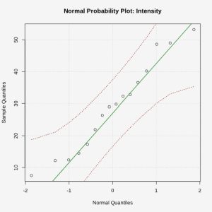
Figure 1: A Normal Probability Plot of Magnetic Intensity The sample data appear to fall along a line, so the assumption that the population is normally distributed is met.
Because we begin the hypothesis test by assuming the null hypothesis is true, we assume the sample is drawn from a population with a mean of
 20 nano-emus and standard deviation of
  14.150 nano-emus. Under these conditions the test statistic is distributed as Student’s t with 15 degrees of freedom.
 - The test statistic is
 .
. - The p-value is the probability of observing a sample mean as extreme as we did under the assumption that the null hypothesis is true. With a statistical program it is simple to conduct a hypothesis test using the value of the t-test statistic. See Figure 2.
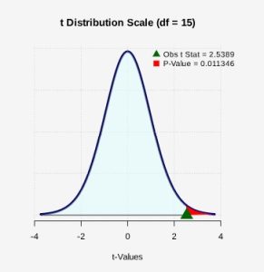
Figure 2: P-value Shaded The p-value is the probability of observing a t-test statistic of t = 2.5389 or more extreme. Because this is a one-tailed (right-tailed) test, the p-value will be calculated by finding the probability as
 0.011346 or approximately 1.1%.
 - Assuming the null hypothesis is true, the probability we would observe a sample mean as extreme as the one we observed is 0.0113. There is a 1.1% chance of observing a sample as least as extreme as we did, which a small probability and less than a 5% level of significance. Because this is highly unlikely, we conclude that we have evidence to reject the null hypothesis. The data supports the claim that the mean magnetic intensity of monarch butterflies exceeds 20 nano-emus. Evidence suggests that monarch butterflies contain a natural magnetic intensity.
Example 2 – Lifespan of Batteries
Imagine that a company sells portable walkie-talkie radios to construction crews. The batteries for these radios last for an average of 55 hours. The purchasing manager for this company receives a brochure in the mail that advertises a new brand of batteries. This new brand of batteries is cheaper than the brand that the company currently uses. However, the purchasing manager is concerned that the cheaper batteries may have a shorter average battery life than the current brand. Note: The number of hours that batteries last is called their battery life. The pricing manager installs 40 randomly selected batteries of the cheaper brand in the company’s walkie-talkie radios. The manager finds that the mean battery life for the sample is 52 hours, with a standard deviation of 10 hours. Perform a statistical test at the 1% level of significance to determine whether the cheaper batteries have a shorter average battery life span than the average life span of the brand of batteries the company currently uses. Assume that the requirement of normality has been met.
Solution:
- The research question involves the mean battery lifetime, so this is a test of means. The alternate hypothesis will state that the mean lifetime is less than 55 hours. The opposite of this claim will be the null hypothesis, that is, the mean lifetime is greater than or equal to 55 hours.
: 
: 
- The study involved a random sample of 40 batteries, with = 52 hours and = 10 hours. We do not have information about the population standard deviation, so we will have to estimate it. As long as the population from which the sample came is approximately normal, the test statistic will be distributed as a t-distribution with 39 degrees of freedom. We are to assume that the population is normally distributed. Because we begin the hypothesis test by assuming the null hypothesis is true, we assume the sample is drawn from a normal population with a mean of 55 hours and standard deviation of 10 hours. Under these conditions the t-test statistic will be used.
- The test statistic is
 .
. - The p-value is the probability of observing a sample mean as extreme as we did under the assumption that the null hypothesis is true. With a statistical program it is simple to conduct a hypothesis test using the value of the t-test statistic. See Figure 3.
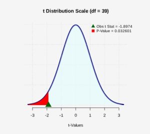
Figure 3: P-value Shaded The p-value is the probability of observing a t-test statistic of t = -1.873 or more extreme. Because this is a one-tailed (left-tailed) test, the p-value will be calculated by finding the probability as
 0.0326 or approximately 3.3%.
 - Assuming the null hypothesis is true, the probability we would observe a sample mean as extreme as the one we observed is 0.0326. There is a 3.3% chance of observing a sample as least as extreme as we did, which a small probability but not less than the 1% level of significance. Because the p-value is larger than the 1% level of significance, we conclude that we do not have enough evidence to reject the null hypothesis. The data do not support the claim that the mean lifetime of batteries is less than 55 hours. The observed sample mean is not statistically significant.
Sources
Statway College Module 4, by Carnegie Math Pathways, is licensed under CC BY NC 4.0.
Douglas Jones and Bruce MacFadden, “Induced Magnetization in the Monarch Butterfly, Danaus Plexippus (Insecta, Lepidoptera)” Journal of Experimental Biology 96 (1982): 1-9.

Feedback/Errata