
3.4 Coefficient of Determination
So far, we have seen how a regression line, or a line of best fit, can be drawn on a scatter plot and used to predict outcomes when a linear relationship is detected between two variables in a given data set or sample. Due to the nature of collecting data, we expect variation, and so far we have concentrated on considering the correlation coefficient and residuals as a way to gain insight into the linear model. The correlation coefficient measures the strength and direction of the linear association between two variables. The residuals, also called errors, measure the distance from the actual value of the response variable and its estimated value. It is the Sum of Squared Errors (SSE), when set to its minimum, which give the regression coefficients for the least-squares regression line.
Once a linear model is created, there are “goodness of fit” statistics that can be used to assess the fit of the model. In this section we will concentrate on the coefficient of determination. As future scientists and engineers, it is important that you focus on the deeper meanings of statistics, so this section will not only explain the meaning behind the coefficient of determination, but it will show you where each part of the calculation comes from, so you will have an appropriate level of understanding of this often misunderstood statistic.
The Coefficient of Determination
The coefficient of determination, denoted as  or
or  , is the square of the correlation coefficient, which we know is denoted as r or R. While correlation is given as a number between -1 and 1, the coefficient of determination is usually given as a percentage. It is very tempting to lump each statistic into the same category and interpret them as statistics that say how good the line fits the data, but this is a very low level interpretation and lacks insight into the incredible amount of information contained in each statistic.
- , when expressed as a percent, represents the percent of variation in the dependent (response) variable that can be explained by variation in the independent (explanatory or predictor) variable using the regression line.
 , when expressed as a percentage, represents the percent of variation in the response variable that is NOT explained by variation in predictor variable using the regression line.
How does a statistic, which is equivalent to the square of the correlation coefficient pull off such an interpretation? It will be worthwhile to demonstrate the creation of the coefficient of determination, so the interpretation is clear. The coefficient of determination partitions several sources of variation. In order to demonstrate the sources of variation, we will use an example with very few data points and visually demonstrate the sources of variation.
Example 1 – Acrylic Paint and Surfactant Use
A surfactant is a liquid that can be added to acrylic paint to reduce the surface tension, thus improving the flow of acrylic paints. Most acrylic paints contain low levels of surfactants, but as water is added into the paint, the need to add additional surfactant increases. A new surfactant is tested by measuring various surfactant concentrations and their corresponding surface tensions. Surface tension is measured in units of millinewton/meter (mN/m), force per unit length. Five data values were taken for different concentrations, with the results given in the following table.
Table 1: Surfactant Concentration and Surface Tension
| Surfactant Concentration % | Surface Tension mN/m |
| 1 | 59 |
| 2 | 55 |
| 3 | 47 |
| 4 | 37 |
| 5 | 35 |
Use a statistical program to create a scatter plot, calculate the correlation coefficient, and the least-squares regression line. Then plot the regression line on the scatterplot.
Solutions:
Because the surface tension is being measured, it is the response variable and will be plotted along the vertical axis. We are checking to see how the response changes as we change the surfactant concentration, so concentration in percent will be plotted along the horizontal axis.
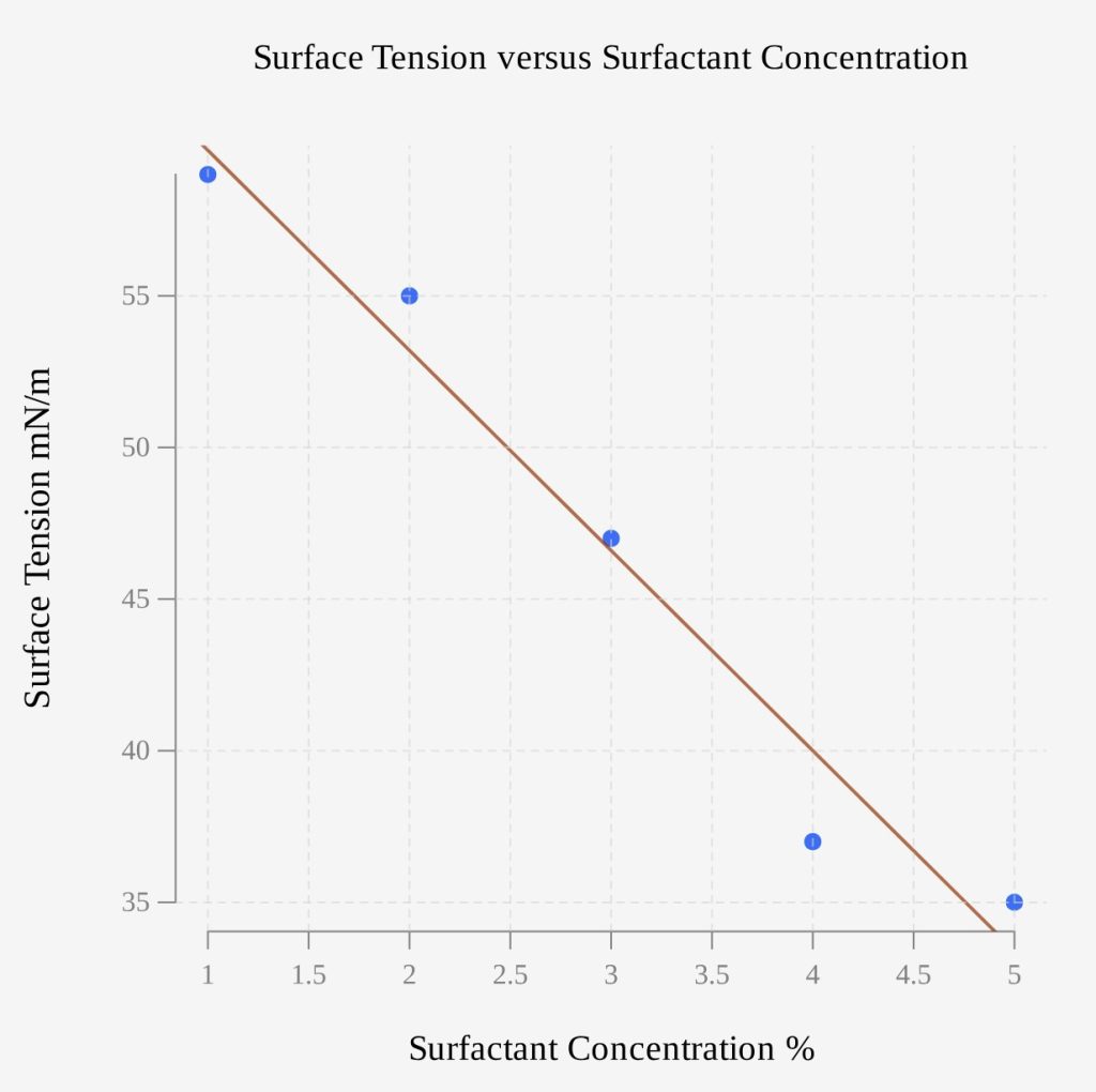
There is a strong negative correlation, with an  . The least-squares linear regression gives the following linear model, with y = surface tension and x = surfactant concentration:
  .
.
SSE – Sum of Squared Errors
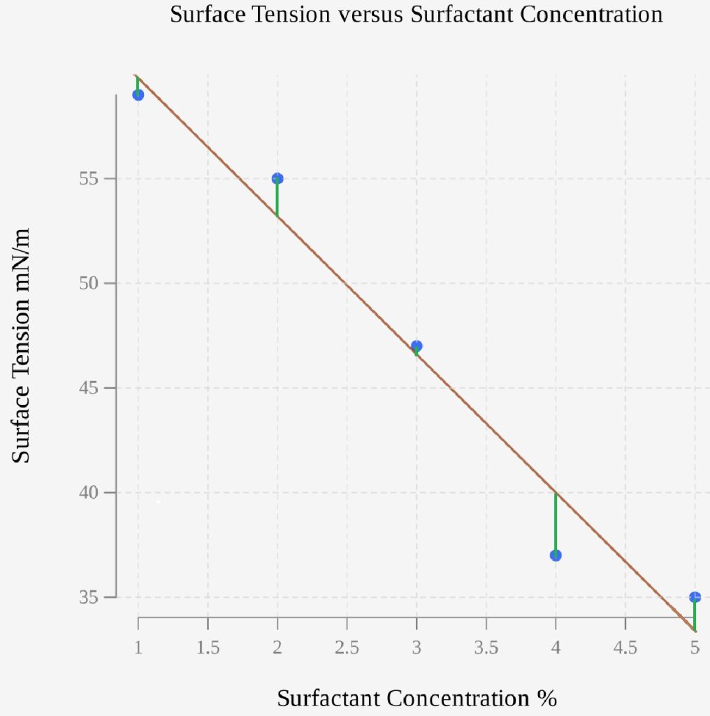
When we use a least-squares linear regression, the regression coefficients minimize the sum of squared errors, SSE. In this case, we have five data points and the linear regression line does not perfectly pass through all five points. Each residual is calculated by subtracting the surface tension observed from the surface tension predicted by the regression line. For each data point the residual can be calculated as  , for i = 1, 2, 3, 4, 5. These calculations are completed in Table 2.
Table 2: Creation of SSE
| Surfactant Concentration %, x | Surface Tension mN/m, y |  |
|
 |
| 1 | 59 | 59.8 | -0.8 | 0.64 |
| 2 | 55 | 53.2 | 1.8 | 3.24 |
| 3 | 47 | 46.6 | 0.4 | 0.16 |
| 4 | 37 | 40.0 | -3.0 | 9.00 |
| 5 | 35 | 33.4 | 1.6 | 2.56 |
| Sum = 15.6 |
Notice in the last column of the table that some residuals are positive and some are negative, so we square them and add them to get  = 15.6 which is the sum of squared errors, SSE. In Figure 2, each residual (the vertical distance from each data value to the value on the regression line) has been drawn in green. The SSE summarizes the sum of the squares of these distances. They visually demonstrate the variation of the original data around the regression line.
SST – Total Sum of Squares
We elected to create the least-squares linear regression based on how well the original data points seemed to follow a linear pattern. What if we did not use a line of best fit at all? If we do not take into account the different levels of surfactant, then we still need to make a single prediction for surface tension based on the data. If we want to make a prediction as to what the surface tension would be in the absence of another changing variable, we already have a way to get our best estimate. We use we the mean. The mean of the original surface tensions is  In Table 3, the difference between each surface tension and the mean is calculated, squared, and added.
  = 451.20. This is called the sum of squares total, SST. It represents the variation around the mean with no other variable taken into account.
Table 3: Creation of SST
| Surfactant Concentration %, x | Surface Tension mN/m, y |  |
 |
 |
| 1 | 59 | 46.6 | 12.4 | 153.76 |
| 2 | 55 | 46.6 | 8.4 | 70.56 |
| 3 | 47 | 46.6 | 0.4 | 0.16 |
| 4 | 37 | 46.6 | -9.6 | 92.16 |
| 5 | 35 | 46.6 | -11.6 | 134.56 |
| Sum = 451.20 |
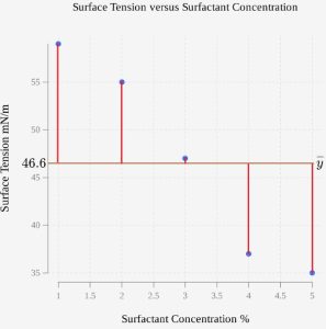
In the absence of any consideration for the surfactant levels, if we draw the distances from the original surface tensions to , we get a visual representation of the total variation around the mean.
SSR – Regression Sum of Squares
We have just considered two important sources of variation, the variation of the data around the mean and the variation of the data around the regression line.
If we consider the difference in these two sources of error, we will get a new statistic:

This difference, SST – SSE = 435.6 has an important meaning. It is a measure of the reduction in variation due to the use of a linear regression. We call this difference the regression sum of squares, SSR. For Example 1, we noticed there was a very large total sum of squares, SST, so the original variation around the mean was large. After the linear regression, we saw the error sum of squares, SSE, was much smaller, so the variation still present after the regression is small. Is an SSR value of 435.6 large or small? If we compare SSR to the total sum of squares, SST, then we get the reduction in variation expresses as a ratio, and we can convert it to a percentage.

We conclude that 96.5% of the total variation in the surface tension data has been reduced by using the linear regression. By taking into account the changing surfactant concentrations, we account for 96.5% of the variation. What we have in our hands right now is the coefficient of determination!
Coefficient of Determination,


Because the total sum of squares, SST, is the sample variance without dividing by  , the coefficient of determination is often described as the proportion of the variance in the response variable explained by regression.
As a final note, we started this section with a few notes about the connection between the correlation coefficient and the coefficient of determination.
Note for Example 1, the correlation coefficient, . When we find the square of the correlation coefficient, we get  . Notice that this is the same as the coefficient of determination we found! While it is easy to calculate the value of the coefficient of determination, the interpretation is much more involved. Much insight can be gained by studying sources of variation!
Sources
Internetagentur, D. T. M. G.-. (n.d.). Surfactants – Measuring the concentration > Measuring surface tension > Applications > SITA Lab Solutions. https://www.sita-lab.com/applications/measuring-surface-tension/surfactants-measuring-the-concentration/

Feedback/Errata