
2.7 Measures of the Spread of Data
An important characteristic of any set of data is the variation in the data. In some data sets, the data values are concentrated closely near the mean; in other data sets, the data values are more widely spread out from the mean. The most common measure of variation, or spread, is the standard deviation. The standard deviation is a number that measures how far data values are from their mean.
Standard Deviation
The standard deviation provides a numerical measure of the overall amount of variation in a data set, and can be used to determine whether a particular data value is close to or far from the mean. Why would we even want this type of information? We already have statistics such as the mean, median, and mode. Unfortunately, they do not tell the whole story of the data. Consider three very small data sets, each of which contain 6 data values.
- Data Set A: 5, 5, 5, 5, 5, 5
- Data Set B: 3, 4, 5, 5, 6, 7
- Data Set C: 1, 2, 5, 5, 8, 9
If you make some quick calculations, you will see that the mean of each data set is 5, the median of each data set is 5, and the mode of each data set is 5. Yet there is something different about these three sets of data that we need to be able to calculate, quantify, and describe. The mean, median, and mode only tell part of the story. We can see that for Data Set A, there is no variation at all, because all the data values are the same. There is, however, some variation in both Data Set B and in Data Set C. You should notice that the variation is greater in Data Set C.
We need a way to describe the idea that the data values are more spread out in Data Set C. Data Set B and C have positive standard deviations but Data Set C has the larger standard deviation of the two.
Deviation From the Mean
If we let x represent a data value, then the difference “x minus the mean” is called its deviation. In a data set, there are as many deviations as there are items in the data set. The deviations for each data value are used to calculate the standard deviation. If the data values belong to a population, then deviations from the mean would look like x – μ. On the other hand, if the data values belong to a sample, then deviations from the mean would look like  . Some deviations will be positive if the data value is greater than the mean and some will be negative if the data value is smaller than the mean.
The procedure to calculate the standard deviation depends on whether the data values make up the entire population or represent just a sample. The calculations are similar, but not identical. Therefore the symbol used to represent the standard deviation depends on whether it is calculated from a population or a sample. The lower case letters represents the sample standard deviation and the Greek letter σ (sigma, lower case) represents the population standard deviation. If the sample has the same characteristics as the population, then s should be a good estimate of σ.
We might think that if we add up all the deviations for a data set, then we would get a single numeric value we could use for the standard deviation, but it is not that simple for one slightly annoying mathematical fact. If we add up all the deviations from the mean for any data set, some deviations will be positive, some negative, and some zero. Added together, the total will always be zero. It is not very useful to get a numeric summary value for a data set that always ends up as zero! In order to get around this issue, we find the deviations first and then we square them to force them to be positive. From there we find the average of these squared deviations, and this measurement actually has a different name. It is called the variance.
Variance
Population
Variance: 
Standard Deviation: 
Sample
Variance: 
Standard Deviation: 
To calculate the standard deviation, we need to calculate the variance first. In words, the variance is the average of the squares of the deviations from the mean. The symbol σ2 represents the population variance; the population standard deviation σ is the square root of the population variance. The symbol s2 represents the sample variance; the sample standard deviation s is the square root of the sample variance. Because we have to square the deviations first to create the variance, the measurement units are squared. After finding the average squared deviation, we find the square root to create the standard deviation, so the standard deviation is a measure of variation that has the same measurement units as the original data. You can think of the standard deviation as a special average of the deviations from the mean.
If the numbers come from a census of the entire population and not a sample, when we calculate the average of the squared deviations to find the variance, we divide by N, the number of items in the population. If the data are from a sample rather than a population, when we calculate the average of the squared deviations, we divide by n – 1, one less than the number of items in the sample. A reason for this is because samples tend to have slightly smaller variation than the population and if we want to use the sample standard deviation to estimate an unknown population standard deviation, then we need to adjust the value up a bit to better estimate the population parameter.
Formulas for the Sample Variance and Standard Deviation
Sample Variance: 
Sample Standard Deviation: 
For the sample standard deviation, the denominator is n – 1, which is one less than the number of items in the sample.
Formulas for the Population Variance and Standard Deviation
Population Variance: 
Population Standard Deviation: 
For the population standard deviation, the denominator is N, the number of items in the population.
Example 1: Calculating the Standard Deviation by Hand
A new reading comprehension teaching strategy will be implemented in a fifth grade class. Before implementing the new strategy, the teacher wanted the statistics related to the average age and standard deviation of the ages of her students. Students entering fifth grade were randomly assigned to her class at the start of the school year, so the 20 students represents a sample of fifth-grade students. The following data are the ages for the 20 fifth grade students, with ages rounded to the nearest half year: 9; 9.5; 9.5; 10; 10; 10; 10; 10.5; 10.5; 10.5; 10.5; 11; 11; 11; 11; 11; 11; 11.5; 11.5; 11.5
Solution:

The average age is 10.53 years, rounded to two places.
The variance may be calculated by using a table. Then the standard deviation is calculated by taking the square root of the variance. An explanation of the columns of calculations is offered after this example.
| Data | Frequency | Deviations | Deviations2 | (Frequency)( Deviations2) |
|---|---|---|---|---|
| x | (freq) | ( x –  ) ) |
( x – )2 |
(freq)(x – )2 |
| 9 | 1 | 9 – 10.525 = –1.525 | (–1.525) 2 = 2.325625 | 1 × 2.325625 = 2.325625 |
| 9.5 | 2 | 9.5 – 10.525 = –1.025 | (–1.025) 2 = 1.050625 | 2 × 1.050625 = 2.101250 |
| 10 | 4 | 10 – 10.525 = –0.525 | (–0.525) 2 = 0.275625 | 4 × 0.275625 = 1.1025 |
| 10.5 | 4 | 10.5 – 10.525 = –0.025 | (–0.025) 2 = 0.000625 | 4 × 0.000625 = 0.0025 |
| 11 | 6 | 11 – 10.525 = 0.475 | (0.475) 2 = 0.225625 | 6 × 0.225625 = 1.35375 |
| 11.5 | 3 | 11.5 – 10.525 = 0.975 | (0.975) 2 = 0.950625 | 3 × 0.950625 = 2.851875 |
| The total is 9.7375 |
The sample variance, , is equal to the total from the last column (9.7375) divided by the total number of data values minus one (20 – 1):  = 0.5125
The sample standard deviation s is equal to the square root of the sample variance: which is rounded to two decimal places, s = 0.72 years.
When the calculation for the standard deviation is completed on a calculator, the intermediate results are not rounded. Rounding is done only at the very last step. This is done for accuracy.
Why not just add up the deviations from the mean?
Looking carefully at the table from Example 1, we note that the deviations from the mean would show how spread out the data are about the mean. Some data values are greater than the mean, so the deviations are positive. Some are less than the mean, so the deviations are negative. The data value 11.5 is farther above the mean than is the data value 11, which is indicated by the greater deviation of 0.97 compared to 0.47. The data value 9 is less than the mean so the deviation is -1.525. You might wonder why we do not just use the sum of all the deviations from the mean as a statistic that could summarize the spread. That is a great idea! However, one property of the deviations from the mean is that if we add up all of the deviations from the mean, we would always get a value of zero! Clearly, that will not be very helpful. So we force the deviations to all be positive by squaring them, which is why you see a deviations squared column in the table.
After we square all the deviations, we will add them all up. We must note the frequency of each data value because each value adds to the variation. By squaring the deviations, they become positive numbers, so the sum will also always be positive. Finally we divide the sum of squared deviations by (n – 1). The variance, then, is the average squared deviation from the mean.
We have the variance, so why do we need the standard deviation?
The variance is a squared quantity and does not have the same units as the data. In Example 1 the sample variance of 0.5125 has units of years squared, which is awkward to interpret. Taking the square root solves the problem. The standard deviation measures the average deviation from the mean and it has the same units as the data. In Example 1, the sample standard deviation is 0.5125 years.
Why do we average the squared deviations by dividing by (n – 1) rather than n ?
Notice that instead of dividing the sum of squared deviations by n = 20, we divided by 19, which is n – 1. We do this when we calculate the sample variance, we always divide by the sample size minus one (n – 1). While this seems strange, there is a reason why we do this. The answer has to do with the population variance. The sample variance is an estimate of the population variance. In general a sample from a population will vary less than the population from which it came. If a goal is to use the sample variance as an estimate of the unknown population variance, we would be using a value that is a little bit too small. As it turns out, dividing by (n – 1) to calculate the sample variance gives a statistic that is a better estimate of the population variance.
Standard Deviation Fun Facts
- Because of the way the standard deviation is calculated, it always takes on a value that is positive or zero.
- The standard deviation is smaller when the data are all concentrated close to the mean, exhibiting little variation or spread.
- The standard deviation is larger when the data values are more spread out from the mean, exhibiting more variation.
- A standard deviation of zero would mean each data value is exactly the same as the mean, so there would be absolutely no variation at all.
- Outliers can make the standard deviation large.
The focus should be on what the standard deviation tells us about the data. The standard deviation is a number which measures how far the data are spread from the mean. Let a calculator or computer do the arithmetic. The standard deviation, when first presented, can seem unclear. By graphing the data, you can get a better feel for the standard deviation. You will find that in symmetrical distributions, the standard deviation can be very helpful but in skewed distributions, the standard deviation may not be very informative. The reason is that the two sides of a skewed distribution have different spreads. In a skewed distribution, it is better to look at the first quartile, the median, the third quartile, the smallest value, and the largest value. As a general rule, always graph your data. Display your data in a histogram or a box plot, so that summary statistics have a visual context.
Relative Position Within a Data Set
Once we have the standard deviation, for any data value, we can calculate how many standard deviations it is above or below the mean. This allows for comparisons of data values within a data set. We could say that a value is within one standard deviation from the mean and you would know that it is close to the mean, but it could be above or below the mean. A value more than three standard deviations above the mean would indicate that the value is much greater than the mean. We often speak of data values by referencing the number of standard deviations above or below the mean. Keep the following formula in mind: value = mean + (#)(standard deviation)
For a sample: x = + (#)(s).
For a population: x = μ + (#)(σ).
For the data we had in Example 1, the sample mean was 10.53 years and the standard deviation was 0.72 years. If we calculate the values that mark 1, 2, and 3 standard deviations, then we have a framework for a description.
- + 1s = 10.53 + (1)(0.72) = 11.25
- – 1s = 10.53 – (1)(0.72) = 9.81
- + 2s = 10.53 + (2)(0.72) = 11.97
- – 2s = 10.53 – (2)(0.72) = 9.09
- + 3s = 10.53 – (3)(0.72) = 12.69
- – 3s = 10.53 + (3)(0.72) = 8.37
For the students in the fifth-grade class we can say, all students between 9.81 years and 11.25 years fall within one standard deviation of the mean. All students between the ages of 9.09 and 11.97 are within two standard deviations of the mean. Those with ages between 8.37 and 12.69 are within three standard deviations of the mean.
Chebyshev’s Rule:
For a set of data, no matter how it is distributed, Russian mathematician Chebyshev discovered the following:
- At least 75% of the data is within two standard deviations of the mean.
- At least 89% of the data is within three standard deviations of the mean.
- At least 95% of the data is within 4.5 standard deviations of the mean.
Example 2
After taking an exam, students are usually curious about how they did, especially relative to the others in the class. Suppose the instructor listed all of the scores: 33; 42; 49; 49; 53; 55; 55; 61; 63; 67; 68; 68; 69; 69; 72; 73; 74; 78; 80; 83; 88; 88; 88; 90; 92; 94; 94; 94; 94; 96; 100
For this data set, verify each of the following:
- The sample mean = 73.5
- The sample standard deviation = 17.9
- The median = 73
- The first quartile = 61
- The third quartile = 90
- IQR = 90 – 61 = 29
A box plot and a frequency histogram have been constructed on the same set of axes. Make comments about the box plot, the histogram, and the chart, especially as it relates to spread.
Answers:
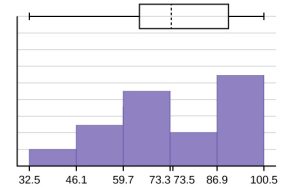 The long left whisker in the box plot is reflected in the left side of the histogram. The spread of the exam scores in the lower 50% is greater (73 – 33 = 40) than the spread in the upper 50% (100 – 73 = 27). The histogram, box plot, and summary statistics all reflect this. There are a substantial number of A and B grades (80s, 90s, and 100). The histogram clearly shows this. The box plot shows us that the middle 50% of the exam scores (IQR = 29) are Ds, Cs, and Bs. The box plot also shows us that the lower 25% of the exam scores are Ds and Fs.
+ 1s = 73.5 + (1)(17.9) = 91.4 and – 1s = 73.5 – (1)(17.9) = 55.6. Of the 31 students, 17 of them earned grades within one standard deviation of the mean. Only one student earned a score more than 2 standard deviations below the mean. – 1s = 73.5 – (2)(17.9) = 37.7.
Comparing Values from Different Data Sets: Z-Score
The standard deviation is useful when comparing data values that come from different data sets as well. However, if the data sets have different means and standard deviations, then comparing the data values directly can be misleading. There is a common way of standardizing the values to make comparisons easy. For each data value, we can calculate how many standard deviations away from its mean the value is in a way that eliminates the measurement units.
For any value, x, use the formula: x = mean + (# of standard deviations)(standard deviation) and solve for # of standard deviations.
# of standard deviations = (x − mean)/(standard deviation)
The result of this calculation is called the z-score and we use the symbol z when we calculate it. In symbols, the formulas become:
For a sample, 
For a population, 
Example 3
Two swimmers, from different teams, each swam the 50-meter freestyle race. Their times were similar but how do they compare to their respective teams? Times are measured in seconds.
| Swimmer | Time | Team Mean Time | Team Standard Deviation |
|---|---|---|---|
| Swimmer 1 | 26.2 | 27.2 | 0.8 |
| Swimmer 2 | 27.3 | 30.1 | 1.4 |
Answer:
For Swimmer 1, the z-score is calculated as z = 
For Swimmer 2, the z-score is calculated as z = 
In this case, faster is better, so swim times below the team average would mean the swimmer is performing better than average. Swimmer 2 had a time that was 2 standard deviations below the team’s mean time. Swimmer 1 had a time that was more than one standard deviation below the team’s mean time. We conclude that Swimmer 2 had the fastest time when compared to her team.
Videos
Calculating the Standard Deviation
Sources
Data from Microsoft Bookshelf.
King, Bill.”Graphically Speaking.” Institutional Research, Lake Tahoe Community College. Available online at http://www.ltcc.edu/web/about/institutional-research (accessed April 3, 2013).
A number that measures, on average, how far data values are from the mean.
When referring to standard deviation, finding the difference between a data value and the mean gives a data value's deviation.

Feedback/Errata