12.2 Shewhart Control Charts for Variables

Shewhart Small Sample Control Charts for Variables

For measurements made on a continuous scale, the data values are called variables data. We will learn to use two types of charts that will help us control the variability in the process and control the process mean, the R Chart and the Xbar Chart. The Xbar and R Charts are charts used together when the sample size is less than or equal to 10. Sampling is a critical step in the control-chart making process. Control charts monitor processes over time, so care must be taken to avoid allowing the sampling technique to introduce additional variation within a sample. Any strategy used for sampling should reduce the within-sample variation as much as possible. This in turn will allow for the detection of the between-sample variation.

Many small samples are taken over time. Each small sample has its own variation, hopefully selected to vary as little as possible (within-sample variation). These are called rational subgroups. Consider for example, a beverage manufacturer and the fill volume of bottles. As filling bottles continues throughout a day, there can be issues with equipment performance, user error, factory temperature, or many other issues which can cause the bottle filling process to wander too far away from what is acceptable and overfill or underfill the bottles. Sampling is carried out that will collect 25 samples of 4 bottles each throughout the day. It is the 4 bottles in each of the 25 samples which make up the rational subgroups. How will those 4 bottles be selected? They could be selected as a set of 4 bottles together from the production every 20 minutes, for example. In this situation, the within-sample variation would likely be small because the bottles collected were produced under nearly the same conditions. Differenced within this group are likely to be random noise (common causes). Because these bottles are collected every 20 minutes, the variation between the rational subgroups, when compared to the within-group variation, can more likely detect a special cause of variation. If the sets of 4 bottles are selected randomly throughout the day, then there is so much production time between the selections, that special causes of variation will likely be a part of the within-group variation, making it harder to detect special causes of variation in the process.

Xbar and R Charts

The Xbar and R Charts are used together. The R Chart measures the within-sample variation. If it is in control, then the Xbar Chart measures the between-sample variation and can reveal any changes in the process.

• The R Chart plots the range of each rational subgroup and displays changes to the within-group variation over time.
• The Xbar Chart plots the mean of each rational subgroup and displays changes to the between-group variation over time.
• Examine the R Chart first. The Xbar Chart control limits rely on the average range values. If the R Chart shows an out of control process, then the Xbar Chart may not be accurate.
• If the R Chart is in control, the review the Xbar Chart.
• If a process is out of control, identify the special cause and address the issue.

Statistics Needed For Variables Control Charts

To construct variable charts, we must know or be able to estimate the process mean and standard deviation, unless standard or target values are provided. We always using at least 25 samples, and assume that our samples are independent and identically distributed, following the normal random variable. For samples, each of size , we produce the following calculations:

Table 1: Statistics Needed for Variables Control Charts

Samples of Size	Mean and Range of Each Sample	Overall Mean and Range
1:  2:  … m:

We assume each of the samples is a sample from a normal distribution with mean and standard deviation . We can refer to these as the process mean and process standard deviation. For each of the samples, the sample mean, , is an approximation to the process mean. The sample range can be used to approximate the process standard deviation, for relatively small samples of up to = 10. For a process which is “in control”, the process mean and process standard deviation are the reasonably the same for each sample. If the process is out of control then several things can happen. In this case, the process mean can be out of control, the process standard deviation can be out of control, or both the process mean and process standard deviation can be out of control.

It is very unusual for most populations to have a value that differs from the mean by more than three standard deviations. A chart that uses this 3 rule is the industry standard and the result is a 3 control chart. The sample mean and the sample range will all vary less when the process is in control, and will tend to stay within the UCL and LCL control limits. An out of control process will more likely show these values exceeding the limits. The UCL and LCL control limits for the Xbar Chart and the R Chart can been estimated using known multiples according to the following information.

For each control chart, the Lower Control Limit (LCL), Center Line (CL), and Upper Control Limit (UCL) are plotted as horizontal lines and then the sample statistics are plotted in order. The details of calculating these control chart limits is given next.

Xbar and R Charts Control Limits

When standards or target values for and are given, set the UCL, CL, and LCL as follows:

Table 2: and Given	Xbar Chart	R Chart
UCL
CL
LCL

When standards for and are not given, and they are estimated from the data, set the UCL and LCL as follows:

Table 3: and Estimated	X Bar Chart	R Chart
UCL
CL
LCL

Table 4: Constants dependent on the size of the rational subgroup.

2	2.121	1.880	1.128	0.853	0	3.266
3	1.732	1.023	1.693	0.888	0	2.574
4	1.500	0.729	2.059	0.880	0	2.281
5	1.342	0.577	2.326	0.864	0	2.114
6	1.225	0.483	2.534	0.848	0	2.003
7	1.134	0.419	2.704	0.833	0.076	1.924
8	1.061	0.373	2.847	0.820	0.137	1.863
9	1.000	0.337	2.970	0.808	0.184	1.816
10	0.949	0.308	3.078	0.797	0.223	1.777

Note: For sample sizes of = 6 or less, the value of is 0. For such small sample sizes the quantity is negative, so the lower control limit is set to 0 due to the fact that it is impossible for the range to be negative.

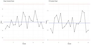
Control charts plot sample values along with the control limits so that it is very easy to see whether the variation signals that the process is out of control. Consider two sample control charts in Figure 1, both generated with the program R. The UCL and LCL are shown as dashed red lines. The process mean is the solid horizontal line. Statistics for each rational subgroup are plotted over time. In this case, both control charts show a process that is in control.

How do we decide whether a process is in control or out of control? It is not enough to verify that samples do not exceed the UCL or LCL. There are other non random patterns that should be considered as well. If certain patterns or trends hang around and persist long enough, then that can indicate a process that is not in control, even if none of the points end up outside of the 3 control limits.

Violations of WECO Rules

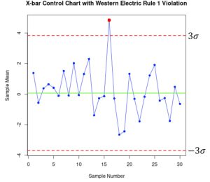
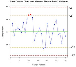
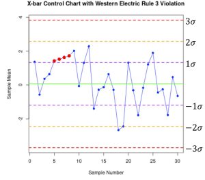
The following three figures demonstrate WECO rule violations samples. Each was generated using the program R. In Figure 2, there is one point identified as exceeding the 3 Upper Control Limit, UCL. This point plotted outside the control limits is evidence that the process is out of control. In Figure 3, there are two out of three consecutive points beyond the 2 threshold. This is a violation of WECO Rule 2. In Figure 4, there is a violation of Rule 4. Notice that there are four out of five consecutive points which exceed 1 from the center line.

Guidelines and Out of Control Behavior

The WECO Rules set guidelines and considerations for trends involving the , , and control limits. For the Xbar Chart and the R Chart, the UCL and LCL control limit formulas are given in Tables 2 and 3. A more generalized, yet equivalent, formula will provide the  needed information for each control limit..

Table 5: General Control Limits

Control Limits	X Bar Chart	R Chart
= UCL
CL
= LCL

If an R Chart is not in control, and there is evidence that a special cause of variation has been operating, then action should be taken to determine the special cause and decide on appropriate action. If a cause is found and a correction is made, then the out of control portion can be deleted and the control chart can be reconstructed and evaluated. Once the process variation is in control, then the process mean can be evaluated with the Xbar Chart. Because the process variation is in control, the process standard deviation is the same for all samples, and can be used to construct the Xbar control limits.

Recalculating Control Limits

Why would we not make adjustments as soon as we see an issue? Since a control chart “compares” the current performance of the process characteristic to the past performance of this characteristic, changing the control limits frequently would negate any usefulness.

So, only change your control limits if you have a valid, compelling reason for doing so. Some examples of reasons:

• When you have at least 30 more data points to add to the chart and there have been no known changes to the process, you get a better estimate of the variability
• If a major process change occurs and affects the way your process runs.
• If a known, preventable act changes the way the tool or process would behave (power goes out, consumable is corrupted or bad quality, etc.)

WECO Rules of Probability

The WECO rules are based on probability. We know that, for a normal distribution, the probability of encountering a point outside is 0.3%, so this is a very rare event. Therefore, if we observe a point outside the control limits, we conclude the process has shifted and is unstable. Similarly, we can identify other events that are equally rare and use them as flags for instability. The probability of observing two points out of three in a row between and and the probability of observing four points out of five in a row between and are also about 0.3%.

False Alarms

While the WECO rules increase a Shewhart chart’s sensitivity to trends or drifts in the mean, there is a severe downside to adding the WECO rules to an ordinary Shewhart control chart that the user should understand. When following the standard Shewhart “out of control” rule, that is, signal if and only if you see a point beyond the plus or minus 3 sigma control limits, you will have “false alarms” every 371 points on the average. Adding the WECO rules increases the frequency of false alarms to about once in every 91.75 points, on the average. The user has to decide whether this price is worth paying (some users add the WECO rules, but take them “less seriously” in terms of the effort put into troubleshooting activities when out of control signals occur).

Sources