
7.2 Estimation, Bias, and Uncertainty
Point Estimation
Suppose you are training for a marathon. Each day you run a different distance. When you take the total distance and divide it by the total time, you get your average time to run a mile. By finding the mean, you create a point estimate of the true mean time it takes you to run a mile.
The most natural way to estimate parameters of the population is to use the corresponding summary statistic, calculated from the sample. Some common point estimates and their corresponding parameters are found in Table 1.
| Parameter | Description | Statistic |
 |
Mean of a single population |  |
 |
Proportion of a single population |  |
 |
Mean difference of two dependent populations (MP) |  |
 |
Difference in means of two independent populations |  |
 |
Difference in proportions of two populations |  |
 |
Variance of a single population |  |
 |
Standard deviation of a single population |  |
Point estimates vary from sample to sample and are almost never exactly equal to the parameter they are estimating. Sometimes they are off by a little and sometimes they are off by a lot. Although variability in samples is present, there exists a fixed value for any population parameter. What makes a statistical estimate of this parameter of interest a good one? It must be both accurate and precise.
Suppose the mean weight of a sample of 60 adults is 173.3 lbs; this sample mean is a point estimate of the population mean weight, µ. Remember this is one of many samples that we could have taken from the population. If a different random sample of 60 individuals were taken from the same population, the new sample mean would likely be different as a result of sampling variability. While estimates generally vary from one sample to another, the population mean is a fixed value.
Suppose a poll suggested the US President’s approval rating is 45%. We would consider 45% to be a point estimate of the true approval rating we might see if we collected responses from the entire population. When the parameter is a proportion, it is often denoted by P, and we often refer to the sample proportion as (pronounced “p-hat”). Unless we collect responses from every individual in the population, P remains unknown, and we use as our estimate of P.
Sampling Distributions
We have established that different samples yield different values of a statistic due to sampling variability. These statistics have their own distributions, called sampling distributions. The sampling distribution of a statistic is the distribution of the point estimates based on many, many samples of a fixed size, n, from a certain population. It is useful to think of a particular point estimate as being drawn from a sampling distribution. It is just one of the possible point estimates we could have observed.
Recall the sample mean weight calculated from a previous sample of 173.3 lbs. Suppose another random sample of 60 participants might produce a different value of the random variable, such as 169.5 lbs. Repeated random sampling could result in additional different values, perhaps 172.1 lbs, 168.5 lbs, and so on. Each sample mean can be thought of as a single observation of a random variable. The distribution of the random variable is called the sampling distribution of the sample mean, and has its own mean and standard deviation like the random variables discussed previously. We will simulate the concept of a sampling distribution using technology to repeatedly sample, calculate statistics, and graph them. However, the actual sampling distribution would only be attainable if we could theoretically take an infinite amount of samples.
Bias
The accuracy of a point estimate refers to how well it estimates the actual value of that parameter. A statistic is an unbiased estimator of the population parameter when the expected value of the statistic is equal to the value of the parameter. Some of the statistics we commonly use are unbiased estimators of the corresponding population parameters. The first unbiased estimator we will consider is the sample mean.
Unbiased Estimator of 
The random variable X has mean  . The sample statistic is an unbiased estimator of , so
  .
.
According to the law of large numbers, probabilities converge to what we expect over time. Point estimates follow this rule, becoming more accurate with increasing sample size. Figure 1 shows the sample mean weight calculated for random samples drawn, where sample size increases by 1 for each draw until sample size equals 500. The dashed horizontal line is drawn at the average weight of all adults 169.7 lbs, which represents the population mean weight according to the CDC.
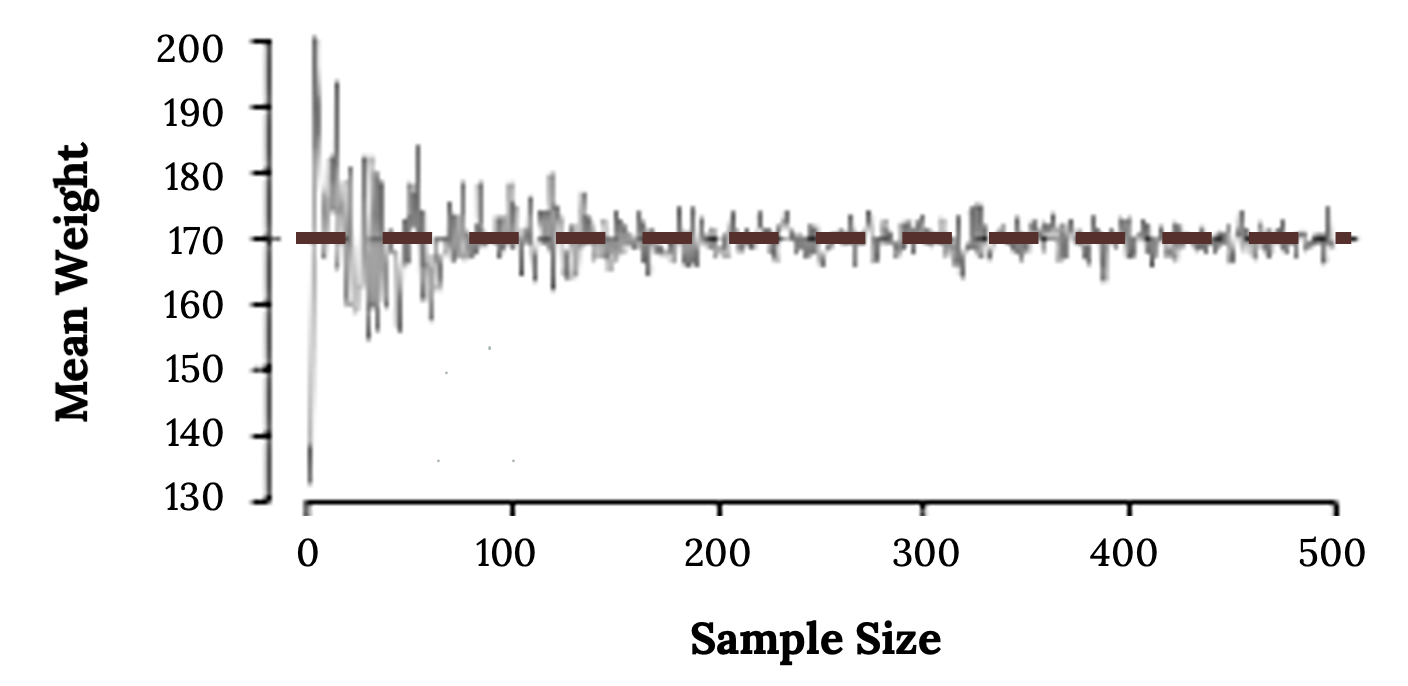
Note how a sample size around 50 may produce a sample mean that is as much as 10 lbs higher or lower than the population mean. As sample size increases, the fluctuations around the population mean decrease; in other words, as sample size increases, the sample mean becomes less variable and provides a more reliable estimate of the population mean.
It might be helpful to think about bias in terms of something many of us do often, that is, weigh ourselves on a scale. A single measurement of weight is not likely to be exactly the true weight of the person. Every measured value will have error. A systematic error, caused by a scale that is not calibrated correctly, will be transferred to every weight in the same way, so that sort of systematic increase or decrease due to a lack of calibration is bias. We can only measure bias if we have a known true value to measure. Every measurement will also have uncertainty. If you step on and off the scale several times and get several weights, they will likely differ from each other. We can gain an estimate in the uncertainty of a weight by taking repeat measurements. This idea is related to precision.
Precision
In addition to accuracy, a precise point estimate is also more useful. When finding repeated measurements, how close to the values resemble each other? When repeatedly sampling or repeatedly taking measurements, if the values seem pretty close together, then the precision is high and uncertainty is low. However, if the repeat measurements differ a lot from each other, then the precision is low and uncertainty is high. For a single measurement, such as a weight from a scale, the estimate of the uncertainty in the measured value is the sample standard deviation. If we consider a statistic such as the sample mean and wonder about its uncertainty, then we must use the standard deviation of the sampling distribution. The phrase “the standard deviation of a sampling distribution” is often shortened to the standard error. A smaller standard error means a more precise estimate and is also affected by sample size, as we will see.
Bias and Uncertainty
- In a single measured value, we can get an estimate of the uncertainty in the measurement by using the sample standard deviation, however, we cannot estimate the bias without knowing the true value of the parameter.
- For a sample mean, we can get an estimate of the uncertainty by using the standard deviation of the sampling distribution, called the standard error, and we know the sample mean is an unbiased estimator of the population mean.
Example 1 – Bias and Uncertainty in Measurements
The former International Prototype of the Kilogram is a cylinder made of platinum and iridium. It was this object whose mass defined the SI unit of mass until the implementation of a revised definition of the kilogram on May 20, 2019. In a lab, the scale is out of calibration. Suppose the former prototype of the kilogram is measured on the scale scale 6 times producing the following measurements, in kilograms: 0.97, 0.98, 0.99, 0.98, 0.97, 0.99. Estimate the bias and uncertainty in a single measurement.
Solution:
Think of the six measurements as a sample of possible measurements taken from a theoretical population of possible measurements for this scale. Because we know the prototype has a mass of exactly 1.00 kilograms, we can estimate the bias in a single measurement. The mean of the sample is 0.98 kilograms and can be used to estimate bias. Because the mean of the sample is not equal to the true value of 1.00 kilograms, we can estimate the bias as 0.02 kilograms. The uncertainty in a single measurement is the standard deviation of the population of possible measurements. We can estimate the uncertainty by using the standard deviation of the six measurements, which is 0.0089 kilograms. Once we recalibrate the scale, we could describe a measurement  0.0089 kilograms. We must have repeat observations to quantify uncertainty.
Sources
Figure 1: Kindred Grey (2020). “Figure 6.3.” CC BY-SA 4.0. Retrieved from https://commons.wikimedia.org/wiki/File:Figure_6.3.pn
IPK – BIPM. (n.d.). BIPM. https://www.bipm.org/en/mass-metrology/ipk

Feedback/Errata