9.3 Hypothesis Z-Test for a Single Mean

Jeff Crabill; Vikki Maurer

9.3 Hypothesis Z-Test for a Single Mean

When our research question involves the population mean, we have knowledge about the population standard deviation, $\sigma$ , and we take a large enough sample, the Central Limit Theorem states that the sample mean is distributed normally. The population from which we are sampling does not have to be normally distributed, but we do need to have prior knowledge of the population standard deviation. How realistic is it to have prior knowledge of the population standard deviation?

In engineering, the frequency of having prior knowledge of the population standard deviation varies depending on the context and the type of data being analyzed. In well-established manufacturing processes, the population standard deviation might be known from historical data. For example, in the production of components with tight tolerances, the variability has likely been studied extensively. Industries with rigorous quality control procedures often have prior knowledge of the standard deviation because they continuously monitor and record data. In highly regulated industries like aerospace, prior knowledge of the population standard deviation is often available because of extensive testing and certification requirements.

However, in new product development, the population standard deviation is often unknown because the process or product is new, and sufficient data has not been collected. In cases such as these, the normal distribution would not be the underlying null distribution. We would have to use the Student’s t-distribution due to having to estimate the population standard deviation.

We begin our work with hypothesis testing by focusing on conjectures about the population mean in situations when we have a large sample and the population standard deviation is known. The type of hypothesis test which applies, in this case, is the z-test.

Z-Test for a Single Population Mean

When performing a hypothesis test involving a single population mean μ, the underlying sampling distribution of the $\bar{x}$ is the normal distribution, as long as a simple random sample was taken, the population standard deviation is know, and the the population is normally distributed or the sample size is sufficiently large for the Central Limit Theorem to apply.

For hypothesis tests involving: $H_o: \mu = \mu_o$ , $H_o: \mu \leq \mu_o$ , or $H_o: \mu \geq \mu_o$ ,

We assume $H_o$ is true, so the null distribution is $\bar{X} \sim N(\mu_o, \frac{\sigma}{\sqrt{n}})$ .

The test statistic (z-score) is $\displaystyle{z = \frac{\bar{x} - \mu_o}{\frac{\sigma}{\sqrt{n}}}}$ .

Probability associated with the test statistic can be found from the standard normal distribution because $z \sim N(0, 1)$ . Equivalently, the p-value can be found using the null distribution directly.

If $H_a: \mu \neq \mu_o$ , calculate the p-value as the sum of the areas in the tails cut off by $-z$ and $z$ .

If $H_a: \mu > \mu_o$ , calculate the p-value as the area to the right of the test statistic, $z$ .

If $H_a: \mu < \mu_o$ , calculate the p-value as the area to the left of the test statistic, $z$ .

Steps to Conducting a Hypothesis Test for a Single Mean:

After considering the research question, define the null and alternate hypothesis statements.
Assume the null hypothesis is true and define the null distribution, stating how assumptions have been met.
Under the assumptions that the null hypothesis is true, calculate the test statistic.
Compute the p-value and create a drawing to support the calculation.
Form a conclusion and write it in the context of the research question.

Example 1 – Are Soda Cans Underfilled?

A quality control engineer plans to take a simple random sample and measure the fill volume of a simple random sample of cans of a soft drink. The cans are supposed to be filled with a 12 ounce volume of liquid. If the cans are being underfilled, then consumers will be unhappy. The engineer wants to test the claim that the cans are being underfilled. The random sample of 35 cans is taken and the sample mean is 11.68 ounces and the sample standard deviation is 0.81 ounces. Through extensive sampling, the population of cans produced is known to have a population standard deviation of 0.89 oz. Conduct the test of hypothesis using the five steps outlined.

Solution:

Create the null and alternate hypothesis statements: The research question involves the mean fill volume, so this is a test of means. Specifically the engineer is wondering if there is evidence to conclude the machine is underfill the cans. The opposite of this claim will be the null hypothesis, that is, that the machine is filling the cans to the desired 12 ounces or more than 12 ounces.
$H_o$ : $\mu \geq 12$
$H_a$ : $\mu < 12$
Determine the underlying null sampling distribution and test statistic: This is a large simple random sample with an interest in the population mean fill volume. Note that in this case, due to prior history with this machine, we can assume the population standard deviation, $\sigma$ = 0.89 oz. Because we begin the hypothesis test by assuming the null hypothesis is true, we assume the sample is drawn from a population with a mean of $\mu_o =$ 12 ounces and standard deviation of $\sigma =$ 0.89 ounces. Under these conditions the sample mean is distributed normally, $\bar{X} \sim N(12, \frac{0.89}{\sqrt{35}})$ and the z-test statistic will be used.
The test statistic is $\displaystyle{z = \frac{\bar{x} - \mu_o}{\frac{\sigma}{\sqrt{n}}}} = \frac{11.68 - 12}{\frac{0.89}{\sqrt{35}}} = -2.1271$ .
The p-value is the probability of observing a sample mean as extreme as we did under the assumption that the null hypothesis is true. With a statistical program it is simple to conduct a hypothesis test using the value of the z-test statistic or, equivalently, with the null sampling distribution directly. Both options are presented in Figure 1:

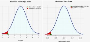
Figure 1: Null Distribution of the Test Statistic and of the Sample Mean

The p-value is the probability of observing a z-test statistic of z = -2.1271 or more extreme. Because this is a one-tailed (left-tailed) test, the p-value will be calculated by finding the probability as $P(z \leq -2.1271) \approx$ 0.0167.
Alternatively, and equivalently, the probability under the null hypothesis of observing a sample mean of $\bar{x}$ = 11.68 ounces or more extreme can be calculated directly as $P(\bar{x} \leq 11.68)$ using the null distribution $\bar{X} \sim N(12, \frac{0.89}{\sqrt{35}})$ . $P(\bar{x} \leq 11.68) \approx 0.0167$ .
Assuming the null hypothesis is true, the probability we would observe a sample mean as extreme as the one we observed is 0.0167. There is a 1.7% chance of observing a sample as least as extreme as we did, which a small probability. Because this is highly unlikely, we conclude that we have evidence to conclude the machine is filling cans to a volume less than 12 ounces.

In Example 1, the soda can fill volume research question involved a one-tailed test. The null hypothesis stated $H_o$ : $\mu \geq 12$ . When the null distribution was considered, it was the value of $\mu_o$ = 12 which was used as the mean of the null distribution. Why did we use 12 ounces rather than any other value less than 12? After all the null hypothesis stated the true mean was hypothesized to be less than or equal to 12 ounces.

Reconsider the sample mean, which was 11.68 ounces. The resulting test statistic (z-score) was more than two standard deviations from $\mu_o$ = 12. If we had used any other null distribution mean, say 11 ounces, 10 ounces, or even smaller, the sample mean would have been even farther away, and the p-value would have been even smaller. So by always using the mean associated with the equality in the null distribution, in this case, 12 ounces, we force the sample to provide the most evidence before we decide to reject the null hypothesis.

Example 2 – Punch Press

Sheet metal punching is the process of creating holes in sheet metal using a punch press. The process involves piercing and cutting the sheet metal, creating holes of various sizes, using dies which are mounted on presses. The machines are designed to create holes with tight tolerances, ensuring that parts fit together perfectly. For a particular machine, circular punches are supposed to have a diameter of 3.4 cm. This process is continuously monitored and the accepted process standard deviation is 0.002 cm. A sample of 35 punches produced a sample mean of 3.401 cm. Conduct a hypothesis test determine if the mean diameter does not specifications, using the five steps outlined.

Solution:

Create the null and alternate hypothesis statements: The research question involves the mean punch diameter, so this is a test of means. Specifically the engineer is wondering if there is evidence to conclude the punch machine is not producing holes with diameter 3.4 cm. The opposite of this claim will be the null hypothesis, that is, that the punch machine is meeting specifications and the mean is 3.4 cm. This is a two-tailed test.
$H_o$ : $\mu = 3.4$
$H_a$ : $\mu \neq 3.4$
Determine the underlying null sampling distribution and test statistic: This is a large simple random sample with an interest in the population mean diameter. Note that in this case, due to prior history with this machine and an acceptable process standard deviation, we can assume the population standard deviation, $\sigma$ = 0.002 cm. Because we begin the hypothesis test by assuming the null hypothesis is true, we assume the sample is drawn from a population with a mean of $\mu_o =$ 3.4 cm and standard deviation of $\sigma =$ 0.002 cm. Under these conditions the sample mean is distributed normally, $\bar{X} \sim N(3.4, \frac{0.002}{\sqrt{35}})$ and the z-test statistic will be used.
The test statistic is $\displaystyle{z = \frac{\bar{x} - \mu_o}{\frac{\sigma}{\sqrt{n}}}} = \frac{3.401 - 3.4}{\frac{0.002}{\sqrt{35}}} = 2.958$ .
The p-value is the probability of observing a sample mean as extreme as we did under the assumption that the null hypothesis is true. Because this is a two-tailed test, if the punch press is out of specification, it could be punching too large or two small, the p-value takes both extreme ends of the null distribution into account $P(z \leq -2.958) + P(z \geq 2.928) = 0.003.$ . See Figure 2 which shows the area representing the p-value probability shaded.

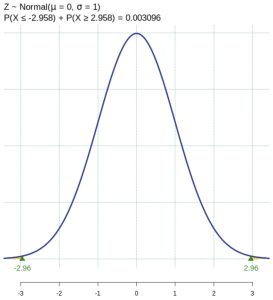
Figure 2: P-Value Diagram
Assuming the null hypothesis is true, the probability we would observe a sample mean as extreme as the one we observed is 0.003. There is a 0.3% chance of observing a sample as least as extreme as we did, which a small probability. Because this is highly unlikely, we conclude that we have evidence to conclude the punch machine is out of specification. We reject the null hypothesis.

Example 3 – Breaking Strength

A manufacturer of a polyester rope used by arborists can withstand an average of 3520 pounds of tension, with a standard deviation of 50 pounds. In order to test the hypothesis that $\mu$ = 3520, against the alternate hypothesis that $\mu > 3520$ , a random sample of 40 ropes will be tested and the null hypothesis will be rejected if the sample mean is greater than 3550 pounds. Find the probability of committing a Type I error.

Solution:

Sampling distribution of the sample mean with the probability of exceeding 3530 shown to be 0.1029. — Figure 3: Probability of a Type I Error

For this hypothesis test, we have the hypothesis statements:

$H_o: \mu = 3520$
$H_a: \mu > 3520$

Because the rejection criterion has been set in advance, we will reject the null hypothesis if the observed sample mean is greater than 3550 pounds. A Type I error is committed if we reject the null hypothesis when it is actually true. So we will find the probability of observing $\bar{x} > 3550$ under the assumption that the null hypothesis is true.

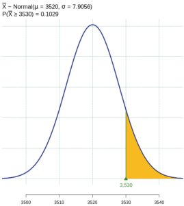
When we assume the null hypothesis is true, we assume $\mu = 3520$ , and the sample mean is distributed as $N( 3520, \frac{50}{\sqrt{40}})$ . Use this normal distribution to calculate $P(\bar{x} > 3550)$ . This probability is shaded in Figure 3 and is 0.1029.