
2.4 Visualizing Data With Boxplots
Boxplots
Boxplots (also called box-and-whisker plots ) give a graphical image of the concentration of the data. They also show how far the extreme values are from most of the data. A boxplot is constructed from five values: the smallest data value, the first quartile, the median, the third quartile, and the largest data value. This is often referred to as the “five-number summary.” We use these values to compare how close other data values are to them.
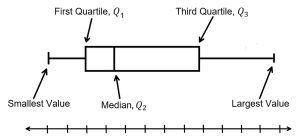
To construct a boxplot, use a horizontal or vertical scaled number line and a rectangular box. The first quartile marks one end of the box and the third quartile marks the other end of the box. The median, or second quartile, can be between the first and third quartiles. The median can be drawn as a solid or dashed line. The “whiskers” extend from the ends of the box to the smallest and largest data values, as shown in Figure 1.
The boxplot gives a good, quick picture of the data. Each boxplot can look very different, depending on the data set. If there are many repeated data values in a data set, it is possible for the first quartile and the median to be the same or for the median and the third quartile to be the same. It is possible for the smallest value to be the same as the first quartile, for example. In cases such as these, there may not be a median line segment marked within the box or there may not be a whisker extending from one end of the box. Every data set is different and the box plot offers a quick visual display that can tell us a lot about how the data is concentrated.
For instance, you might have a data set in which the median and the third quartile are the same. In this case, the boxplot would not have a dotted line inside the box displaying the median. The right side of the box would display both the third quartile and the median. For example, if the smallest value and the first quartile were both 1, the median and the third quartile were both 5, and the largest value was 7, the boxplot would look like Figure 2.

In this case, when the smallest value and the first quartile are the same, we would know at least 25% of the values are equal to one. Further, because the median and the third quartiles are the same, 25% of the data values are between 1 and 5, inclusive, and at least 25% of the values are equal to five. The top 25% of the values fall between 5 and 7, inclusive.
Example 1
Consider a set of 14 data values, which have already been organized from smallest to largest. Construct a boxplot of the data.
1, 1, 2, 2, 4, 6, 6.8, 7.2, 8, 8.3, 9, 10, 10, 11.5
Answer: You should verify that the smallest value is 1 and the largest value is 11.5. The first quartile is 2, the median is 7, and the third quartile is 9. The following image shows the constructed boxplot.

The two whiskers extend from the first quartile to the smallest value and from the third quartile to the largest value. The median is shown with a dashed line. Notice how the scaled number line makes it easy to read off the corresponding values of the statistics that make up the boxplot.
Once we organize the data from smallest to largest and determine the quartiles, we can assess whether there are outliers. A generally accepted rule for defining an outlier is a data value that is 1.5(IQR) greater than the third quartile or 1.5(IQR) below the first quartile. When an outlier is discovered, we mark them with a dot or symbol and the whisker extends to the first non-outlier value instead.
Example 2
Narrow-spectrum antiepileptic drugs (AEDs) are designed to treat specific kinds of seizures. In one study, the number of seizures per month was recorded for 15 patients testing a new AED. Create a box-and-whisker plot for the data values shown and denote any outliers with a dot. Then write a summary of the information provided by the boxplot.
Number of Seizures per Month: 0, 5, 5, 15, 30, 30, 45, 50, 50, 60, 75, 110, 140, 240, 330
Answer: The data are in order from least to greatest. There are 15 values, so the eighth number in order is the median: 50. There are seven data values less than the median and 7 values to the right. The five values that are used to create the boxplot are:
Five-Number Summary: Smallest Value = 0, Q1 = 15, Median = 50, Q3 = 110, Largest Value = 330
Notice that the IQR is Q3 – Q1 = 110 – 15 = 95. If we consider possible outliers we calculate 1.5(IQR) = 1.5(95) = 142.5. Because the first quartile is 15, there are no data values smaller than Q1 – 1.5(IQR). Consider the third quartile. When we calculate Q3 + 1.5(IQR), we see 110 + 1.5(95) = 252.5, and note that any data value greater than 252.5 is considered an outlier value. There is one data value greater than 252.5. The patient who had 330 seizures in a month is considered an outlier. It is an extreme value and is denoted with a dot. We must avoid assuming any outlier is a mistake. The outlier is a data value that may need additional scrutiny but we do not eliminate outliers unless there is a clear reason to do so.
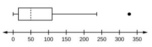
Notice that the upper 50% of seizures displays a greater spread then the lower 50%. Half of the patients experienced at most 50 seizures in a month. About half of the patients experienced between 50 and 240, with one patient having 330 seizures in one month.
We have already learned how to calculate the first quartile, median, and third quartile for a data set, so we should now focus on interpreting a finished boxplot. What generalizations can we make once the boxplot is constructed?
Example 2
The following data are the heights of 40 individuals who require a knee replacement. These heights are arranged from smallest to largest.
59 60 61 62 62 63 63 64 64 64 65 65 65 65 65 65 65 65 65 66 66 67 67 68 68 69 70 70 70 70 70 71 71 72 72 73 74 74 75 77
Verify the five-number summary and boxplot construction. Then list as much information as you can think of that you gain from studying the boxplot.
Answer:
- Smallest Value = 59
- Largest Value = 77
 : First Quartile = 64.5
 : Second Quartile or Median = 66
 : Third Quartile = 70

- Each quarter has approximately 25% of the data.
- The spreads of the four quarters are 64.5 – 59 = 5.5 inches for the first quarter, 66 – 64.5 = 1.5 inches for the second quarter, 70 – 66 = 4 inches for the third quarter, and 77 – 70 = 7 inches for the fourth quarter. So, the second quarter has the smallest spread and the fourth quarter has the largest spread.
- The range is calculated as largest value – the smallest value = 77 – 59 = 18, so the range is 18 inches.
- The interval 59–65 has more than 25% of the data, so it has more data in it than the interval 66 through 70 which has 25% of the data.
- Interquartile Range: IQR = Q3 – Q1 = 70 – 64.5 = 5.5 inches.
- The middle 50% (middle half) of the data has a range of 5.5 inches.
Comparing Boxplots
Constructing side-by-side boxplots offer an effective way to visually compare data sets. When creating a side-by-side boxplot, use one scaled number line for reference.
Example 3
An education specialist is studying the effects of using collaborative learning groups on test scores. The scores for the class which used the collaborative learning groups are listed as well as test scores for a control group.
Control Class Scores: 99 56 78 55.5 32 90 80 81 56 59 45 77 84.5 84 70 72 68 32 79 90
Collaborative Learning Class Scores: 98 78 68 83 81 89 88 76 65 45 98 90 80 84.5 85 79 78 98 90 79 81 25.5
- Find the five-number summary for the control class.
- Find the five-number summary for the collaborative learning class.
- Create a boxplot for each set of data. Use one scaled number line for both box plots.
- Which boxplot has the widest spread for the middle 50% of the data? What does this mean for that set of data in comparison to the other set of data? What other observations can be made?
Answer:
- Min = 32, Q1 = 56, Median = 74.5, Q3 = 82.5, Max = 99
- Min = 25.5, Q1 = 78, Median = 81, Q3 = 89, Max = 98
- The boxplot for the control class is on top:
Image description. - The control class has the wider spread for the middle 50% of the data. The IQR for the control class is greater than the IQR for the collaborative learning class. This means that there is more variability in the middle 50% of the scores for the control class. Notice that the collaborative learning class has a higher median compared to the control. At least 50% of students in the collaborative learning class scored at least 81 compared to 74.5 for the control class. At least 75% of the students in the collaborative learning class scored higher than 50% of the control class.

Example 4
The following data set shows the heights in inches for the boys and for the girls in a class of 40 students.
Heights of Boys: 66; 66; 67; 67; 68; 68; 68; 68; 68; 69; 69; 69; 70; 71; 72; 72; 72; 73; 73; 74
Heights of Girls: 61; 61; 62; 62; 63; 63; 63; 65; 65; 65; 66; 66; 66; 67; 68; 68; 68; 69; 69; 69
Construct a side-by-side boxplot and provide an explanation for the information the boxplots provide.
Answer:

Notice that the IQR for the boys = 4 inches while the IQR for the girls = 5 inches. The boxplot for the heights of the girls has the wider spread for the middle 50% of the data. Notice for the boys, the heights in the upper 50% of the data were more variable, while for the girls, the heights in the lower 50% were more variable. All of the boys are taller than 50% of the girls.
Videos
YouTube Video Box and Whisker Plot
Additional Resources – Technology
Use the online imathAS boxplot tool to create box and whisker plots.
Image Descriptions
Description 1
Horizontal boxplot box begins at the smallest value and Q1, 1, until the Q3 and median, 5, no median line is designated, and has its lone whisker extending from the Q3 to the largest value, 7. Return to image.
Description 2
Horizontal boxplot’s first whisker extends from the smallest value, 1, to the first quartile, 2, the box begins at the first quartile and extends to the third quartile, 9, a vertical dashed line is drawn at the median, 7, and the second whisker extends from the third quartile to the largest value of 11.5. Return to image.
Description 3
Horizontal boxplot with first whisker extending from smallest value, 59, to Q1, 64.5, box beginning from Q1 to Q3, 70, median dashed line at Q2, 66, and second whisker extending from Q3 to largest value, 77. Return to image.
Description 4
Two box plots over a number line from 0 to 100. The top plot shows a whisker from 32 to 56, a solid line at 56, a dashed line at 74.5, a solid line at 82.5, and a whisker from 82.5 to 99. The lower plot shows a whisker from 25.5 to 78, solid line at 78, dashed line at 81, solid line at 89, and a whisker from 89 to 98. Return to image.
A figure which separates data into quartiles using a box and lines extending from the box, called whiskers. A scaled number line is used for reference.
A data value that is much larger or smaller than the rest of the data values. One generally accepted formula to test if a data value is an outlier is to see if it is at least 1.5(IQR) greater than the third quartile or 1.5(IQR) smaller than the first quartile.

Feedback/Errata