8.1 Introduction: Confidence Intervals

We use inferential statistics to make generalizations about unknown properties of a population. The simplest way of doing this is to use the sample data help us to make a point estimate of a population parameter. We learned that the sample mean, , is a point estimate for the population mean, . The sample proportion, , is a point estimate for the population proportion, . While these statistics are helpful, they are single numbers and are not likely equal to the population parameter they are estimating.

Due to sampling variation, the point estimate can be very close to the parameter it is estimating, and we hope it is, but it can also be far from the parameter. Because of this, offering the point estimate alone is not enough. We need to also offer some sense of how far off our estimate might be. For point estimates that have a normal distribution, we have a way of indicating the uncertainty in the estimate. After calculating point estimates, we can build off of them to construct interval estimates, called confidence intervals.

A confidence interval is another type of estimate but, instead of being just one number, it is an interval of numbers. It provides a range of reasonable values in which we expect the population parameter to fall. Essentially the idea is that since a point estimate may not be perfect due to variability, we will build an interval based on a point estimate to hopefully capture the parameter of interest in the interval. There is no guarantee that a given confidence interval does capture the parameter, but there is a predictable probability of success for the confidence interval method.

Confidence Interval Overview

A confidence interval is another type of estimate but, instead of being just one number, it is an interval of numbers. The interval of numbers is a range of values calculated from a given set of sample data. The confidence interval process gives us confidence that the interval produced contains the unknown population parameter. Keep in mind that once an interval is created, the interval will or it will not contain the true population parameter. At that point there is no probability statement that can be made. Probability is reserved for statements about future events. We will build confidence intervals using a method, so that if we produced many confidence intervals, most of them would contain the true population parameter. We hope the one we use is one of those, but as always with statistics, we might get one of the intervals that does not contain the parameter.

Suppose, for example, that a new process is used to produce pickleball paddles with a target weight of 8 oz. After a production run of several thousand paddles, a sample of 100 paddles is taken producing a sample mean of = 7.95 oz and sample standard deviation = 0.31 oz. We do not know the true mean, , of the population of manufactured paddles, but we do recall the Central Limit Theorem, so we know how the random variable, , is distributed.

By the Central Limit Theorem, we know the sample mean has a normal distribution with mean, , and standard error, . The standard error for the sample mean requires knowledge of the population standard deviation, but we can use the sample standard deviation to estimate it. Thus, .

The empirical rule, which applies to in this case, says that in approximately 95% of samples from a normal distribution, a randomly selected value of the random variable will be within two standard deviations of the mean. The sample mean is a random variable, so 95% of sample means will be within two standard errors (standard deviation of the sample mean) of the mean .

The Empirical Rule

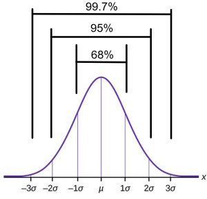
If X is a random variable and has a normal distribution with mean µ and standard deviation σ, then the Empirical Rule says the following is true of every normal distribution:

• About 68% of the population will fall within one standard deviation of the mean, or .
• About 95% of the population will fall within two standard deviations of the mean, or .
• About 99.7% of the population will fall within three standard deviations of the mean, or .

These percentages of the population that fall within one, two, or three standard deviations is the same for any normal distribution. (See Figure 1.)

For our pickleball paddle example, two standard errors is roughly (2)(0.031) = 0.062. We would have confidence then that the sample mean  oz is within 0.062 oz of . We create the confidence interval by adding and subtracting this value from the sample mean. The lower number is calculated by taking the sample mean and subtracting two standard errors (2)(0.031) and the upper number is calculated by taking the sample mean and adding two standard errors. In other words, μ is between 7.95 − (2)(0.031) = 7.89 oz and 7.95 + (2)(0.031) = 8.01 oz in 95% of all the samples, so the confidence interval is presented as (7.89, 8.01).

When we calculated two standard errors, we created something called the margin of error. So, μ is likely to be within 0.062 oz units of in 95% of the samples.  We would have a high level of confidence to state the true mean weight of the production of pickleball paddles as or as the interval from  7.89 oz to 8.01 oz. 

Notice that we use careful language with confidence intervals. We say we have “95% confidence” that the unknown population mean paddle weight is between 7.89 oz and 8.01 oz. We do not say, “There is a 95% probability.” With any confidence interval there are only two possibilities once the interval is constructed. Either the interval contains the true mean μ or it does not. Once the interval is created, we can state only that we are 95% confident.

A confidence interval is created to find a range of possible values for an unknown population parameter, such as the population mean, μ. One of the decisions that must be made before constructing a confidence interval is how confident we want to be. We will rely on the empirical rule for confidence levels. The confidence level will give a multiplier, called the critical value, for the standard error, and together they make up the margin of error. In general the confidence intervals we shall study have the following form:

When you read newspapers and journals, some reports will use the phrase “margin of error.” Other reports will not use that phrase, but include a confidence interval as the point estimate plus or minus the margin of error. These are two ways of expressing the same concept.