6.5 The Normal Distribution

Jeff Crabill; Vikki Maurer

6.5 The Normal Distribution

The normal distribution, which is a continuous distribution, is arguably the most important of all the distributions. It is widely used and even more widely abused. Its graph is bell-shaped and most people recognize it from that characteristic bell shape. However, having a bell shape is not enough to say that a distribution is actually normal. There are other requirements as well. You see the normal distribution in almost all disciplines. Some of these include psychology, business, economics, the sciences, nursing, and, of course, mathematics. Some of your instructors may use the normal distribution to help determine your grade. Most IQ scores are normally distributed, as well as heights, weights, and errors, to specify a few. Often real-estate prices fit a normal distribution. The normal distribution is extremely important, but it cannot be applied to everything in the real world.

We will study the normal distribution as one of our continuous probability distributions. We will also discuss and work with the standard normal distribution.

The Normal Probability Distribution

This is a frequency curve for a normal distribution. It shows a single peak in the center with the curve tapering down to the horizontal axis on each side. The distribution is symmetrical; it represents the random variable X having a normal distribution with a mean, m, and standard deviation, s. — Figure 1: Normal Distribution

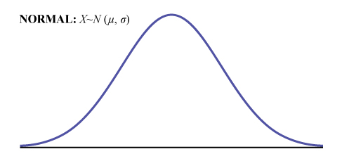
The normal distribution has two parameters that determine its shape, the mean (μ) and the standard deviation (σ). (See Figure 1.) If X is a quantity to be measured that has a normal distribution with mean (μ) and standard deviation (σ), we designate this by writing $X \sim N(\mu, \sigma)$ .

The probability density function, PDF, for a normal distribution is given by

$f(x)=\frac{{1}}{{\sigma\sqrt{2\pi}}}\cdot{e}^{{-}\frac{{1}}{{2}}\cdot{\left(\frac{{x-\mu}}{{\sigma}}\right)}^{2}}$

Just as we have with other continuous probability distributions, we need to calculate probabilities. We have already used integration for other continuous probability distributions to find the areas under their PDFs. It is worth a few minutes right now for you to take a close look at the PDF for the normal distribution. While the PDF has several parts, note that symbols $\mu$ , $\sigma$ , and of course $\pi$ are all constants. If we (just for a moment) ignore all those constants, notice that the core function is exponential: $e^{-x^2}$ . Think about how you might integrate $\int_{-\infty}^{\infty} {e}^{-x^{2}}dx$ . You might want to try a u-substitution, but it would fail. What about integration by parts? Nope. Fail. Try every technique you have learned and you will conclude that this is not a function that can be integrated. The fundamental theorem of calculus guarantees the antiderivative exists, but we do not have a foundational function that is the antiderivative. This is why we will have to use approximation techniques or statistical software to calculate areas associated with any normal distribution.

Normal Distribution Probabilities

The Normal Probability Distribution Function cannot be integrated by conventional integral calculus means. Numerical integration must be used (e.g. Simpson’s Rule) or other approximation methods. To that end, we use technology to compute probabilities for us. Before so many tools were available, statisticians relied on tables of probabilities. Common tools you can use include the following:

Rguroo
Excel or Google sheets
Desmos
Any TI graphing calculator
Various internet calculators

You are encouraged to learn how to compute probabilities in this chapter using several of these tools.

Any normal PDF curve is symmetrical about a vertical line drawn through the mean, μ. In theory, the mean is the same as the median, because the graph is symmetric about μ. As the notation indicates, the normal distribution depends only on the mean and the standard deviation. Since the area under the curve must equal one, a change in the standard deviation, σ, causes a change in the shape of the curve. The curve becomes fatter or skinnier depending on σ. A change in μ causes the graph to shift to the left or right. This means there are an infinite number of normal probability distributions.

Normal Random Variable

If the random variable, X, is distributed normally, then we use the notation, $X \sim N(\mu,\sigma)$ .

The probability density function is $f(x)=\frac{{1}}{{\sigma\sqrt{2\pi}}}\cdot{e}^{{-}\frac{{1}}{{2}}\cdot{\left(\frac{{x-\mu}}{{\sigma}}\right)}^{2}}$

The mean is $\mu$ .

The standard deviation is $\sigma$ .

We mentioned that not every bell-shaped curve is normal, so let’s discuss the additional requirements in order to say we have a normal distribution.

The Empirical Rule

Bell shaped curve with the mean and one, two, and three standard deviations above and below the mean marked. The percentage of the distribution between one, two and three standard deviations are marked as 65%, 95%, and 99.7% as described in the text. — Figure 2: Empirical Rule

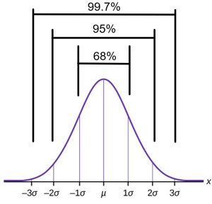
If X is a random variable and has a normal distribution with mean µ and standard deviation σ, then the Empirical Rule says the following is true of every normal distribution:

About 68% of the population will fall within one standard deviation of the mean, or $\mu \pm \sigma$ .
About 95% of the population will fall within two standard deviations of the mean, or $\mu \pm 2\sigma$ .
About 99.7% of the population will fall within three standard deviations of the mean, or $\mu \pm 3\sigma$ .

These percentages of the population that fall within one, two, or three standard deviations is the same for any normal distribution. (See Figure 2.) You may have heard the expression of some measurement being “within one standard deviation of the mean.” This would mean an event or measurement is very usual. Almost 70% of observations from a normal distributions fall within one standard deviation of the mean. On the other hand, it is highly unusual to observe a value from a normally distributed population which is more than three standard deviations away from the mean. Knowing a z-score gives information about how usual or unusual an event might be.

Example 1 – Grade on a Curve?

Students in an engineering class received their test scores and were not happy with their letter grades. The 24 student scores were: 49, 50, 55, 57, 58, 59, 60, 65, 66, 67, 68, 69, 70, 73, 74, 75, 76, 81, 82, 83, 84, 90, 91, 92. Based on a traditional way to assign letter grades, the instructor announced scores below 60 earned an F; scores between 60 and 69 earned a D; scores between 70 and 79 earned a C; scores between 80 and 89 earned a B; and scores of at least 90 earned an A. The students were not happy that there were 6 Fs, 6 Ds, 5 Cs, 4 Bs, and 3 As. They asked the instructor to please “grade on a curve.”

Take on the role of the instructor, and assume the students want you to grade on a normal curve. Show how many scores would fall within one, two, and three standard deviations of the mean according the Empirical Rule. Let C grades fall within one standard deviation of the mean. Let D and B grades fall outside the C range but within two standard deviations of the mean, and let F and A grades fall outside of that. Who will be happy or unhappy over this new curve?

Solution:

According to the Empirical Rule, 68% of the scores would earn a C grade. For this class of 24 students, that amounts to (0.68)(24) = 16.32. The middle 16 scores would be assigned a C grade.

To form the next grade cutoffs, consider the 95% range of (0.95)(24) = 22.8. If we remove the 16.32 who are already earning a C grade, then we see 6.48 would earn a D or a B, so 3 scores would be assigned a D and 3 scores would be assigned a B.

The remaining two scores would be the most extreme and would earn the F and A grades.

The new letter grades are as follows:

F Grade: 49

D Grade: 50, 55, 57

C Grade: 58, 59, 60, 65, 66, 67, 68, 69, 70, 73, 74, 75, 76, 81, 82, 83

B Grade: 84, 90, 91

A Grade: 92

After reviewing these letter grades, the students at the bottom were likely happy because they ended up in higher grade categories compared to traditional cutoffs. The students who traditionally earned B and A grades were not happy that the curve forced most of them into a lower grade category.

Because the normal distribution is so common, there is a tendency to think everything is normal, but we now know it is not the case. However, when we do have normally distributed data, it is very common to standardize measurement units so we make comparisons. Each population will have a different mean, standard deviation, and measurement units, however, if we standardize the information, then we can compare populations more easily.

Z-Scores

If X is a normally distributed random variable and $X \sim N(\mu, \sigma)$ , then the z-score is calculated as

$\displaystyle{z}=\frac{{x - \mu}}{{\sigma}}$

The z-score tells you how many standard deviations the observed value x is above (to the right of) or below (to the left of) the mean, μ. Values of x that are larger than the mean have positive z-scores, and values of x that are smaller than the mean have negative z-scores. If x equals the mean, then x has a z-score of zero. Notice that the measurements for the value of the random variable, the mean, and the standard deviation are all the same, and cancel away in the calculation of the z-score. In this way, the z-score is a unitless number that summarizes the standardized distance from the mean.

Example 2 – Bolts Wrong Size

In June of 1990, a pilot of a British Airways airplane on flight 5390 was sucked out of the cockpit and pinned to the outside of the airplane after a windshield came off of the airplane. The pilot did survive the event. After studying the incident, it was determined that 84 of the 90 bolts used to secure the windshield were too small in diameter. These 84 bolts were supposed be part number (A211-8D), with a mean diameter of 0.188 inches and a standard deviation of 0.0005 inches. Instead these 84 bolts were part number (A211-8C), with diameters ranging from 0.1605 inches to 0.1639 inches. (See the Aircraft Incident Report.)

Determine the bolt sizes for part number (A211-8D) that would correspond to z-scores of -3 and 3 and summarize what the Empirical Rule suggests about these bolt diameters.
If the investigator did not know that the 84 bolts actually used were a completely different part number and assumed the 84 bolts were from the the correct batch, what would the z-score be for a bolt diameter of 0.1639 inches? Comment on the likelihood of observing such a diameter.

Solutions:

The population from which the bolts should have come had a mean diameter of 0.188 inches and a standard deviation of 0.0005 inches.
For a z-score of -3, the corresponding bolt diameter, x, is found by solving: $-3 =\frac{x - 0.188}{0.0005}$ , so x = 0.1865 inches.
For a z-score of 3, the corresponding bolt diameter, x, is found by solving: $3 =\frac{x - 0.188}{0.0005}$ , so x = 0.1895 inches.The Empirical Rule suggests that if bolt diameters are normally distributed, then 99.7% of the bolts will have a diameter between 0.1865 inches and 0.1895 inches.
The z-score of a 0.1639 inch diameter bolt is $z=\frac{0.1639 - 0.188}{0.0005} = -48.2$ . A z-score more than 3 standard deviations from the mean suggests a very unlikely observation. This z-score is -48.5, which suggests the bolt was from a completely different population of bolts. This is in fact what happened!

Example 3 – Tensile Strengths

The tensile strength of a material is the maximum amount of load the material can support, when being pulled or stretched, without fracture. An engineer is tasked with comparing the tensile strength of a certain type of material produced using two different manufacturing processes. Tensile strength measurements, in megapascals (MPa), from both processes are collected. For process A, tensile strengths have a mean of 520 MPa with a standard deviation of 20 MPa. Process B yields a mean of 470 MPa with a standard deviation of 25 MPa.

Sample tensile strength measurements yield 490 MPa from process A and 500 MPa from process B. Calculate and compare the z-scores.

Solutions:

The sample from process A has a z-score of $z=\frac{490 - 520}{20} = -1.5$ . Note that this tensile strength is 1.5 standard deviations below the mean.

The sample from process B has a z-score of $z=\frac{500 - 490}{25}= 0.4$ . Note that this tensile strength is 0.4 standard deviations above the mean.

It is difficult to compare raw data values from two different populations. Calculating the z-scores allows for each each sample to be compared to its own mean and standard deviation.

Standard Normal Distribution

The parameters for a normal distribution, which affect the location and shape, are the mean and standard deviation. Each mean and standard deviation produce a different normal distribution. With technology, we can and will find probabilities related to each individual normal distribution easily. It is handy, however, to understand and use a standardized normal distribution. The standard normal distribution is a normal distribution of standardized values, which we know are called z-scores. Probabilities related to the standard normal distribution have been extensively calculated, and by calculating z-scores for a data value, it is easy to get a sense of where that value falls within the distribution.

The mean for the standard normal distribution is zero, and the standard deviation is one. For a random variable $X \sim N(\mu, \sigma)$ , the transformation $\displaystyle{z}=\frac{{x - \mu}}{{\sigma}}$ produces the distribution $Z \sim N(0, 1)$ .

Example 4 – Standardized Normal Distribution

According to the CDC National Center for Health Statistics, the body mass index, BMI, of male 10-year-old children during the years 2015 to 2018 has a mean of 20.1 and a standard deviation of 5.3. BMI gives values in terms of $\frac{kg}{m^2}$ . If we assume BMI is normally distributed and the population of 10-year old males has $\mu$ = 20.1 and $\sigma$ = 5.3, and we select two 10-year-old boys and find their BMI are 18.2 and 29.5, then convert these to standardized units.

Solutions:

For this population we can visualize the normal distribution with a mean at 20.1 and standard deviation of 5.3. We can mark off each one standard deviation departure from the mean and those would correspond to z-scores ranging from -3 to 3.

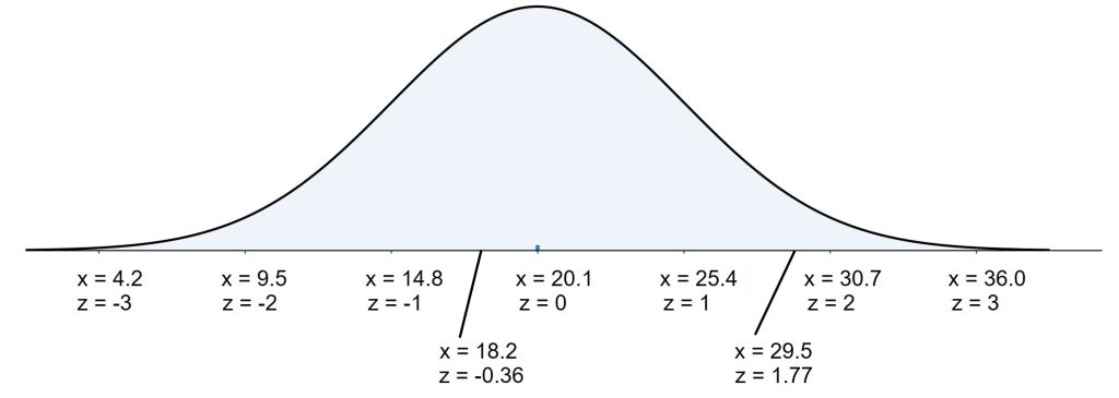
A normal curve labeled with the given mean and standard deviation as well as the standardized values as described in the text.

The z-score for a BMI value of 18.2 is $z = \frac{18.2 - 20.1}{5.3} = -0.36$ . By standardizing the value, we can see this BMI is below average but within one standard deviation of the mean.

The z-score for a BMI value of 29.5 is $z = \frac{29.5 - 20.1}{5.3} = 1.77$ . We see this BMI is more than one standard deviation above the mean.

Normal Distributed or Not and Why Care?

In many areas, we have so much practice with certain types of data, that we can assume a population is normally distributed. If we do not know for sure, then we must rely on the sample to decide if the population from which the sample was drawn is normal. Why does it even matter? As we move forward in statistics and we explore ways to draw conclusions and conduct tests of hypotheses, we will rely on processes which are built on the assumption that the underlying population is normally distributed. If we use a statistical process with a population that is not actually normally distributed, then conclusions are potentially meaningless.

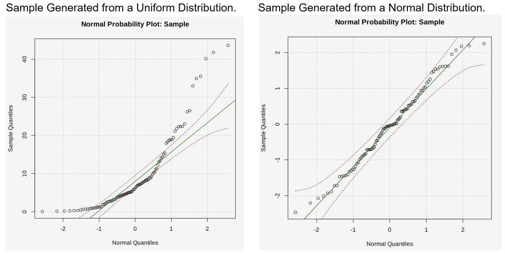
One observation you may have already made involving the normal distribution, after reading about the Empirical Rule, is that normal distributions rarely contain outliers. This is why we always look at the data and graphs, such as histograms, generated from the data first. We look for outliers and consider symmetry and shape. While a visual inspection is an important starting point, we may not want to rely just on our visual assessment of a histogram, however. A version of the Q-Q Plot (Quartile-Quartile) is a plot we can use in which the quantiles of a data set are plotted against the quantiles of a normal distribution. This special Q-Q Plot is also called a Normal Probability Plot. If the data fall along a line, especially between the first and third quantiles, then it indicates the data comes from a normal distribution.

To illustrate the Q-Q Plot, consider two sets of data, each generated from a different theoretical population. One data set contains 100 values randomly generated from an exponential distribution. The other data set contains 100 values randomly generated from a normal distribution. For each, a Q-Q Plot was created to assess the normality of the data. These plots are presented in Figure 3: Q-Q Comparison Plots. In these plots, if the data come from a normal distribution, then the data, especially in the middle quantiles, should fall closely along a line with no systematic departure from the line. Notice the severe and consistent departures from the line with the exponentially distributed data, while the middle portion of the normally distributed data closely follows the line. There are challenges involved in visually inspecting such a plot. This is why there are tests that we can rely on as well.

Two normal probability plots, one for exponential data and one for normal data to demonstrate what the plots look like. — Figure 3: Q-Q Comparison Plots

There are many tests for normality often used today, two of which are the Kolmogorov-Smirnov Test for Normality and the Shapiro-Wilk test. These tests each compare the data to a normal distribution and create a single number to use as a guide for deciding if the data is from a normally distributed population.

Kolmogorov-Smirnov Test: The Kolmogorov-Smirnov (K-S) test is considered to be a less powerful test and compares the observed distribution of a dataset to a specified theoretical distribution, in this case, the normal distribution. The test calculates the maximum difference between the two cumulative distribution functions. A large maximum difference indicates a significant deviation from normality. One limitation of the K-S test is that it is less sensitive to deviations in the distribution’s tails.

Shapiro-Wilk Test: The Shapiro-Wilk test is a powerful normality test. It is specifically designed for small to moderate sample sizes. The test calculates a W statistic, which compares the observed data to the expected data if it follows a normal distribution. A small W value indicates that the data deviates significantly from a normal distribution.

These sorts of tests and tools are available and as you move forward in your study of statistics, you will encounter them and will need to use them. It is best to rely on multiple assessments, such as a visual inspection of a histogram as well as Q-Q plot along side of any normality test.

Videos

YouTube Video Normal Distribution

YouTube Video Standard Normal Distribution

YouTube Video Normal Distribution Part 2

Sources

Hardiman, J., & Mitchell, A. (2023, December 4). The pilot that survived 20 minutes outside a flying jet in 1990. Simple Flying. https://simpleflying.com/british-airways-flight-5390/

Department of Transport, Aircraft Incident Report 1/92, (1992) Report on the accident to BAC One-Eleven, G-BJRT over DIDcot, Oxfordshire on 10 June 1990. https://assets.publishing.service.gov.uk/media/5422faa7e5274a131400078d/1-1992_G-BJRT.pdf

CDC, National Center for Health Statistics, National Health and Nutrition Examination Survey. https://www.cdc.gov/nchs/data/series/sr_03/sr03-046-508.pdf

License

Icon for the Creative Commons Attribution 4.0 International License

Introduction to Statistics for Engineers Copyright © by Vikki Maurer & Jeff Crabill & Linn-Benton Community College is licensed under a Creative Commons Attribution 4.0 International License, except where otherwise noted.

Feedback/Errata

Comments are closed.