
5.5 Poisson Distribution
The Poisson Probability Distribution
In science and engineering, we are often concerned with the number of events occurring in a fixed interval of time or space. Because we are considering a number of events, the random variable involved will be a count, and the probability distribution will be discrete. Consider processes in manufacturing where the rate of flaws in the product is known. If we are interested in the number of flaws in a given period of time, then the Poisson distribution governs this situation.
There are three main characteristics of a Poisson experiment or process.
- The Poisson probability distribution gives the probability of a number of events occurring in a fixed interval of time or space.
- The events happen with a known average rate, λ, which is a positive constant.
- Each event happens independently of the time since the last event.
Poisson Probability Density Function
The random variable X = the number of occurrences of the event in the interval of interest.
If X ~ Poisson(λ), then the probability density function is given below:

Note: x is a nonnegative integer.
The mean is  .
.
The variance is  .
.
Note: The Poisson distribution may be used to approximate the binomial if the probability of success is “small” (such as 0.01) and the number of trials is “large” (such as 1000). You will verify the relationship in the homework exercises. n is the number of trials, and p is the probability of a “success.”
Example 1 – Historic Flooding
Over the last 60 years, the Willamette River in Oregon has experienced 6 historic flooding events, so the rate of historic flooding is 6 floods per 60 years. If we assume this rate is fixed and historic flooding events occur independently (these are big assumptions that would need investigating), then what is the probability there will be 2 historic flood events in the next 10 years?
Answer:
If we define the random variable X as the number of historic floods in 10 years, and we know the average rate is  , then λ = 0.1. The probability there will be 2 historic flooding events in the next 10 years is expressed as P(X = 2), where X ~ Poisson(0.1).
P(X = 2) =  , so there is about a 0.45% chance of there being exactly two historic floods of the Willamette River in the next 10 years.
Example 2 -Internet Interruption
There were 6 interruptions to Internet service between 8 a.m. and 10 a.m. What is the probability there will be more than one interruption in the next 15 minutes?
Answer:
Let  the number of Internet interruptions in 15 minutes. Notice that the interval of interest in this case is 15 minutes or
  hour. We know there are 6 interruptions in a 2 hour period. A 2-hour period contains eight 15-minute intervals, so the mean rate of interruption is
  and we define λ = 0.75. Therefore,
  .
.
The probability there will be more than one interruption in the next 15 minutes is expressed as  and is best calculated by using the complementary event.
![\begin{align*} P(X > 1) &= 1 - P(X \leq 1) \\ &= 1 - \left[P(X=0) + P(X = 1)\right] \\ &= 1 - \left[(e^{-0.75} \enspace \frac{0.75^0}{0!}) + e^{-0.75} \enspace \frac{0.75^1}{1!} \right] \\ &= 1 - \left(0.47236 + 0.35427 \right) \\ &\approx 0.1734 \end{align*}](https://openoregon.pressbooks.pub/app/uploads/quicklatex/quicklatex.com-9035d7d24bd0b0951caa35988f5fc464_l3.png "Rendered by QuickLaTeX.com")
There is approximately a 17.34% chance that there will be more than one Internet interruption in the next 15 minutes.
The probability histogram of is:
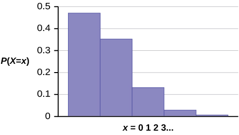
The y-axis contains the probability of x where the number of calls in 15 minutes.
Example 3 – Porch Pirates
In Albany, Oregon during December, an average of 147 packages per day are stolen from residential porches. Let X represent the number of packages stolen per day. The discrete random variable X takes on the values  0, 1, 2 …. The random variable X has a Poisson distribution with a mean of 147 packages per day.
 .
.
- What is the probability that no packages will be stolen in a day?
- What is the probability that more 125 packages will be stolen in a day?
Answer:
 . There is almost no chance of no packages getting stolen in a day in December.
 . There is approximately a 96.45% chance of more than 125 packages being stolen in Albany on a December day.
Poisson Approximation of the Binomial
A Poisson probability distribution of a discrete random variable gives the probability of a number of events occurring in a fixed interval of time or space, if these events happen at a known average rate and independently of the time since the last event. The Poisson distribution may be used to approximate the binomial, if the probability of success is “small” (less than or equal to 0.05) and the number of trials is “large” (greater than or equal to 20).

Feedback/Errata