
5.2 Discrete Probability Distribution Function
Probability Distributions of Discrete Random Variables
Engineers often encounter systems and phenomena that exhibit inherent variability, whether it’s in manufacturing processes, environmental conditions, or communication channels. Understanding random variables is crucial for engineers as it provides them with the tools to model and analyze this variability mathematically. By studying random variables, engineers can develop probabilistic models that capture the uncertainties present in their systems, allowing for more robust designs, accurate predictions, and informed decision-making. Whether optimizing production processes, designing communication systems resilient to noise, or assessing structural safety in varying environmental conditions, a deep understanding of random variables equips engineers with the necessary framework to tackle real-world challenges effectively.
Random Variable Definition
A random variable is a rule or a function which assigns a numeric value to each of the possible outcomes of an experiment. If the outcomes are countable then the random variable is discrete. If the outcomes are measured then the random variable is continuous.
When we make a list of the possible values the random variable can take on along with the probability each value can occur, we create a probability distribution function, or PDF for short.
A discrete probability distribution function has two characteristics:
- Each probability is between zero and one, inclusive.
- The sum of the probabilities for all possible outcomes is one.
Discrete Probability Distribution Function
If X is a discrete random variable, and if for each possible outcome, x, of the random variable,


then the set of ordered pairs (x, P(x)) makes up a discrete probability distribution function, also called just the probability distribution or PDF.
Example 1 – Verify Discrete Probability Distribution Function
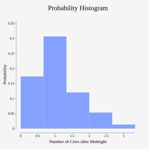
A child psychologist studying newborn babies, within the first seven days of life, and is interested in the number of times per week a newborn cries after midnight. For a random sample of 50 newborns, the following information was obtained. Verify the information in the table is a discrete probability distribution function.
Let the random variable X = the number of times per week a newborn baby cries after midnight. In this study, the babies observed cried between 0 and 5 times after midnight during a week. Note: P(x) = probability that the random variable X takes on a value x.
| x | P(x) |
|---|---|
| 0 | P(x = 0) = 2/50 |
| 1 | P(x = 1) = 11/50 |
| 2 | P(x = 2) = 23/50 |
| 3 | P(x = 3) = 9/50 |
| 4 | P(x = 4) = 4/50 |
| 5 | P(x = 5) = 1/50 |
X takes on the values 0, 1, 2, 3, 4, and 5. These are all positive counted values. The relative frequency or probability each occurred is listed as P(x). Note that if we add up each of the probabilities, we get 2/50 + 11/50 + 23/50 + 9/50 + 4/50 + 1/50 = 1.
This is a discrete PDF because:
- Each P(x) is between zero and one, inclusive.
- The sum of the probabilities is one.
| x | P(x) |  |
|---|---|---|
| 0 | P(x = 0) = 2/50 |  = 2/50 = 2/50 |
| 1 | P(x = 1) = 11/50 |  = 13/50 = 13/50 |
| 2 | P(x = 2) = 23/50 |  = 36/50 = 36/50 |
| 3 | P(x = 3) = 9/50 |  = 45/50 = 45/50 |
| 4 | P(x = 4) = 4/50 |  = 49/50 = 49/50 |
| 5 | P(x = 5) = 1/50 | = 50/50 = 1 |
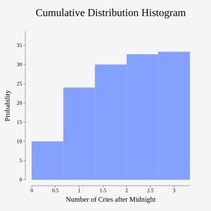
Cumulative Distribution Function
For a discrete random variable X, with probability distribution given by P(X = x), the cumulative distribution function is given by
F(x) = 
for each possible outcome x.
Inference in statistics involves drawing a sample from a population and studying the sample data so that conclusions and inference can be made about the population. In many situations, the probability density function can be well approximated or categorized as a standard known function. We will encounter several of these standard density functions in this class. Consider a situation in which there is one trial or one observation and there are exactly two outcomes. This is a very special case of a known random variable.
A Common Discrete Random Variable
A Bernoulli Random Variable or Bernoulli “trial” is a two option, “yes or no” random variable. The two options are often referred to as “success” or “failure” in the definition with one of them labeled as 1 and the other labeled as 0. It has one parameter p, which denotes the probability of observing the success. For engineers, the choice of assigning probabilities to success or failure is arbitrary. Often, however, in engineering a “success” is similar to the idea of “true”, which is labeled as 1 in any digital logic class. A Bernoulli random variable is named for Jacob Bernoulli who, in the late 1600s, studied them extensively.
Bernoulli Distribution
If X is a Bernoulli random variable, its probability distribution is

Thus a Bernoulli random variable can take on only the values X = 0 or X = 1. The parameter p is the probability that the random variable is 1. This makes the probability that the random variable is 0 equal to 1 – p, so most often, we will see P(X = 1) = p and P(X = 0) = 1 – p. The random variable is said to have a Bernoulli Distribution with parameter, p. An often used notation for random variables involves naming them and placing the parameter in parentheses.

When we flip one coin exactly one time, we are performing a Bernoulli trial. We can assign the observation of a heads as 1 or 0, depending on which one we want to call a success. If the coin is fair, and if we agree that observing tails is defined as a success, then  .
.

Feedback/Errata