
3.5 Residual Plots
We have seen how the method of least-squares linear regression produces a best-fitting line by minimizing the sum of the squared residuals, SSE. We also saw how the sum of squared residuals, along with the total sum of squares, created the coefficient of determination, used in quantifying the percentage of variation accounted for by using the linear model. We have done all this work with linear models, but how can we be confident the linear model was the best one to use in the first place? What if another model, one we have not considered, would do a better job? One way to assess whether a linear model is appropriate is by creating and analyzing a residual plot.
Residual Plot
A residual plot is a scatterplot that displays the relationship between the residuals of the line of best fit,  , and the fitted values,
  . The fitted values are on the horizontal axis and the residuals are on the vertical axis.
Example 1 – Expenditures in Health Care
Over the past two decades, the amount of money spent on health care by both individuals and the government in the United States increased dramatically. This spending has also had an effect on the overall growth rate of the U.S. economy. The scatterplot below shows health care expenditures, that is, what we in the United States have spent on health care, over an 11-year time period. The scatterplot also shows the least-squares regression line for the data. (Source: Centers for Medicare & Medicaid Services.)
The least-squares linear regression line has been calculated as  , where x represents the number of years since 1994.
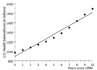
- Do you think the linear regression line is an appropriate model for predicting health care expenditures during the 11-year time period. Why or why not?
- By how much does the line of best fit predict that health care expenditures will change each year?
- When looking at the scatter plot, does the change in expenditures from year to year stay consistent?
- Previously we learned that the residual is the distance between a point in the scatterplot and the regression line. Points above the line have positive residuals and points below the line have negative residuals. Do you notice any pattern in the residuals of the data points? What is the pattern?
Answers:
- In this case, there is a distinct curve to the scatterplot. A linear model may not be the best model to use.
- The slope of the linear model is 92.1, so for each year between 1994 and 2005, the model predicts a 92.1 billion increase in expenditures.
- The increase in expenditures from data value to data value stays fairly constant for the years from 1994 to 1998. After that time, the annual increase grows causing the curved tendency.
- The residuals for the first three years and the last three years are positive. The other residuals for the middle years are negative.
In Example 1, a problem was detected in the scatter plot. We fit a best-fitting line to the scatter plot but there was a curved trend in the data. Consider the data in Table 1. The original data values are given along with the predicted values from the least-squares regression line and the residual for each data value.
Table 1: Residuals for National Health Care Expenditures between 1994 and 2005
|
Year After 1994 |
Expenditures (billions) |
Predicted Value |
Residual |
|---|---|---|---|
|
x |
y |
|
|
| 0 | 972.5 | 893.7 | 78.8 |
| 1 | 1,027.3 | 985.8 | 41.5 |
| 2 | 1,081.6 | 1077.9 | 3.70 |
| 3 | 1,142.4 | 1170.0 | -27.6 |
| 4 | 1,208.6 | 1262.1 | -53.5 |
| 5 | 1,286.8 | 1354.2 | -67.4 |
| 6 | 1,378.0 | 1446.3 | -68.3 |
| 7 | 1,495.3 | 1538.4 | -43.1 |
| 8 | 1,637.0 | 1630.5 | 6.5 |
| 9 | 1,772.2 | 1722.6 | 49.6 |
| 10 | 1,894.7 | 1814.7 | 80.0 |


Example 2 – Residual Plot for Health Expenditure Data
Use the residuals from Table 1, for the health expenditure data between the years 1994 and 2005 to create a plot of the residuals on the vertical axis and the fitted values along the horizontal axis. Comment on any trends or patterns you see in the residual plot.
Solution:
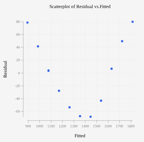
The residual plot shows a clear curve with the first three residuals and the last three residuals positive. All the others are negative.
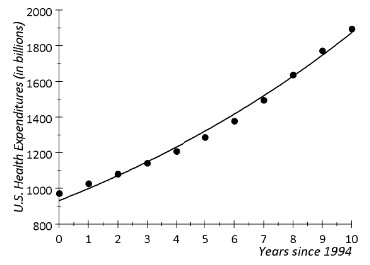
Sometimes a pattern is observed in the residual plot of a linear regression model. When there is a pattern, a line may not be the best model of the relationship between the explanatory and response variables. When this occurs, a nonlinear model may lead to more accurate predictions. Why do we even need a residual plot if we can see the curved trend without it? There are times when issues with a scatter plot will be hard to discern just by looking with your eyes. The residual plot exaggerates the vertical deviations to show more detail than can be detected in the original scatter plot.
In the case of the national health care expenditures data, a curved model more appropriately describes the relationship. The graph in Figure 3 shows the health care expenditures data with a curved mathematical model.
Issues With a Residual Plot
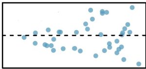
Patterns: There should not be a clear pattern in a residual plot, such as a curve or a wavy tendency as shown in Figure 4. An acceptable residual plot will show no clear pattern.
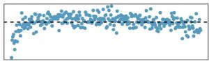
Variation Increase or Decrease: There should not be any systematic increase or decrease in variation as shown in Figure 5. The variation in the residuals should look roughly uniform throughout the plot. Variance that changes is this way is considered to show heteroscedasticity. For least-squares regression, the variance in the residuals should show homoscedasticity, which means there should be constant variance.
Keep in mind that having a residual plot with none of these issues does not all by itself mean that a linear model is appropriate. However, when we see a residual plot with issues, we can conclude that a linear model is not appropriate.
Example 3 – Ohm’s Law Linear Regression with Residual Plot
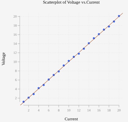
In an engineering laboratory, engineers are testing the relationship between voltage (V) and current (I) in an electrical circuit. Ohm’s Law states that the current flowing through a conductor is directly proportional to the voltage applied across it. They suspect a linear relationship between these variables based on these theoretical expectations and initial experiments. To validate their hypothesis, they conduct experiments where they measure voltage across a resistor for different values of current. Each data point represents a pair of measurements: one for voltage and one for current.
Current (Amperes): 1, 2, 3, 4, 5, 6, 7, 8, 9, 10, 11, 12, 13, 14, 15, 16, 17, 18, 19, 20
Voltage (Volts): 1.2, 2.1, 2.9, 4.2, 4.9, 6.1, 7.1, 7.9, 9.2, 10.2, 11.1, 11.8, 12.9, 14.1, 15.2, 16.1, 17.1, 17.8, 18.9, 20.1
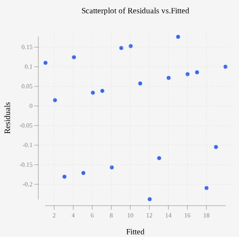
Use a statistical program to create a scatter plot, linear regression model, and residual plot. Then comment on the validity of the linear model.
Solution:
A scatter plot with current as the predictor variable and voltage as the response variable shows a strong linear trend. The correlation value is 0.99973 and the least-squares regression line is given as  . The residual plot shows no systematic curvature or change in variation. A linear model appears to be appropriate.
Summary
- The sum of squared residuals is used to create the least-squares regression line.
- The line of best fit produces the smallest possible SSE for any linear model. Another name for the line of best fit is the least squares regression line for this reason.
- Patterns in the residuals can be seen more clearly in a residual plot than in a scatter plot of the data alone.
- Patterns indicate that a nonlinear model may be appropriate or a transformation of the data is needed.
Sources
CC BY-NC 4.0 Deed | Attribution-NonCommercial 4.0 International | Creative Commons. (n.d.). https://creativecommons.org/licenses/by-nc/4.0/
Diez, D., Cetinkaya-Rundel, M., & Barr, C. (2022). OpenIntro Statistics (4th ed.), Creative Commons BY-SA 3.0 license

Feedback/Errata