
3.2 Scatter Plots and Correlation
Before we take up the discussion of linear regression, we need to examine a way to display the relation between two variables. The most common and easiest way is a scatter plot. The following example illustrates a scatter plot.
Example 1 – M-Commerce Retail Sales
M-commerce is the buying and selling of goods and services using mobile devices. M-commerce is a subset of e-commerce and has grown tremendously worldwide. For the years 2015 through 2021, did there appear to be a relationship between the year and smartphone retail sales? Construct a scatter plot. Let x = the year and let y = the retail sales, in billions. Comment on the scatterplot and the relationship between the variables.
| Year | Retail Sales in Billions of Dollars |
| 2015 | 37.72 |
| 2016 | 67.25 |
| 2017 | 102.14 |
| 2018 | 146.26 |
| 2019 | 200.81 |
| 2020 | 262.80 |
| 2021 | 333.65 |
Solution:
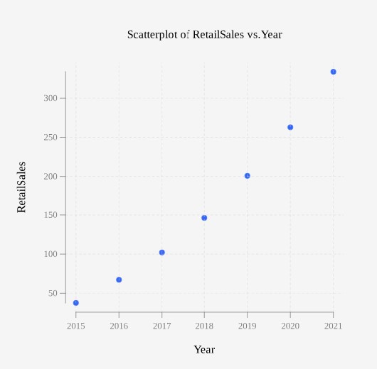
As time passes, it does appear that there is a relationship between the year and retail sales. Retail sales increase each year. In this case there is a curve in the relationship suggesting there is an increase in growth each year compared to the year before.
A key idea to focus on involves what we do once we notice that there appears to be a relationship between two variables. How will we describe it and how will we quantify it? Can we use it to make a prediction into the future? Take another look at the trend in the scatterplot of Example 1. If we were to decide that the relationship between year and retail sales appears to be linear and use a linear function to make a prediction about what the retail sales would be in 2025, then we might have a prediction that is way off. In this case the relationship appears to have a curved trend and projecting into the future would offer incorrect predictions, but that is always a risk we take if we try to project too far into the future based on data.
A scatter plot shows the direction of a relationship between the variables. The direction can be positive or negative. A positive association happens when there are high values of one variable occurring with high values of the other variable and low values of one variable occurring with low values of the other variable. This was the case in Example 1, with the year and retail sales. Another way the direction of the relationship can show up is to see high values of one variable occurring with low values of the other variable. This would be a negative association.
You can determine the strength of the relationship by looking at the scatter plot and seeing how close the points are to a linear function, a power function, an exponential function, a sinusoidal function, or to some other type of function. The relationship can be strong, weak, or there can be no discernable relationship at all.
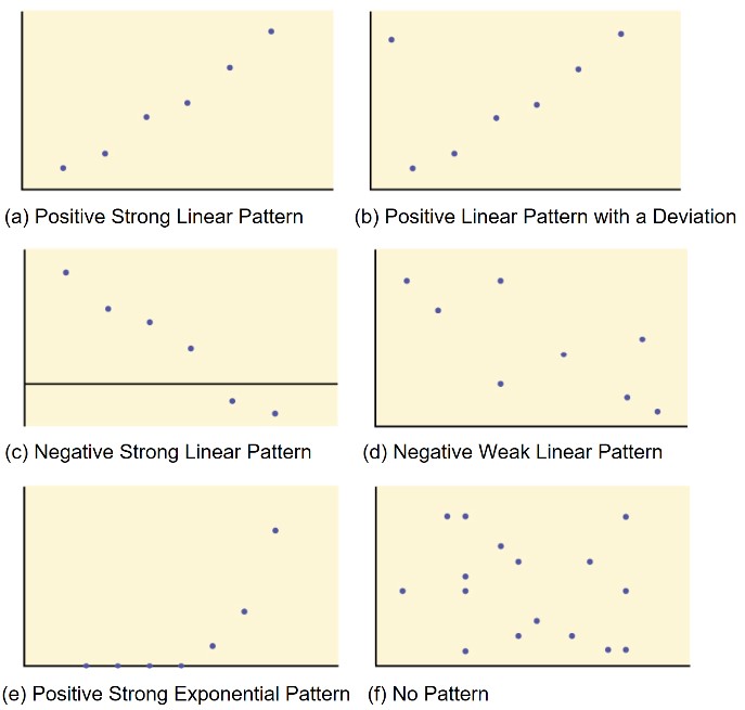
When looking at a scatterplot, notice the overall pattern and any deviations from the pattern. The following six scatterplot examples in Figure 1 illustrate these concepts.
In this chapter, we are interested in scatter plots that show a linear pattern. Linear patterns are quite common. The linear relationship is strong if the points are close to a straight line, with a non-zero slope. If we think that the points show a linear relationship, we would like to draw a line on the scatter plot to mimic the trend we see. We can certainly use a hand-drawn line that seems to fit the data pretty well, but there has to be a more systematic way to get a good fitting line and even the best fitting line. There is in fact such a method. We will learn a process of creating a line which is calculated through a process called least-squares linear regression. However, we only calculate a regression line if one of the variables helps to explain or predict the other variable. If x is the independent variable and y is the dependent variable, then we can use a regression line to predict a value of y for a given value of x.
Outliers
As we noted in a previous section, the IQR (Inner Quartile Range) can help to determine potential outliers in a data set. A value is suspected to be a potential outlier if it is less than (1.5)(IQR) below the first quartile or more than (1.5)(IQR) above the third quartile. Potential outliers always require further investigation and thoughtful consideration.
The Correlation Coefficient
Besides looking at the scatter plot and seeing that a line seems reasonable, how can you tell if the line is an appropriate model? Use the correlation coefficient as another indicator of the strength of the linear relationship between two variables.
The correlation coefficient, r, developed by Karl Pearson in the early 1900s, is single number which provides a measure of strength and direction of the linear association between the independent variable x and the dependent variable y. There are several equivalent formulas for the correlation coefficient. In general, we will use a statistical program to calculate the correlation but it is worth taking a close look at the formula to get a sense of what it is calculating.
One formula for the correlation coefficient gives insight into what the statistic is calculating, where n is the number of data points.

- Notice the z-scores for x and y are multiplied and averaged.
- Notice that when data values for x and y are each greater than their means at the same time, the product will be positive, and when less than the mean at the same time, the product will be positive. Otherwise, the product will be negative. In this way the positive trend or negative trend of the linear relationship becomes apparent in the sign of the correlation.
- The correlation coefficient is unitless due to the numerators and denominators having the same units. Thus the correlation will not be affected by the measurement units of the underlying data sets.
Another equivalent version of the formula is easier to use if calculating the correlation coefficient by hand.

What the VALUE of r tells us: The value of r is always between –1 and +1, in other words –1 ≤ r ≤ 1. The size of the correlation indicates the strength of the linear relationship between x and y. Values of r close to –1 or to +1 indicate a stronger linear relationship between x and y. If r = 0 there is absolutely no linear relationship between x and y (no linear correlation). If r = 1, there is perfect positive correlation. If r = –1, there is perfect negative correlation. In both these cases, all of the original data points lie on a straight line. Of course, in the real world, this will not generally happen.
What the SIGN of r tells us: A positive value of r means that when x increases, y tends to increase and when x decreases, y tends to decrease (positive correlation). A negative value of r means that when x increases, y tends to decrease and when x decreases, y tends to increase (negative correlation). The sign of r is the same as the sign of the slope of the best-fitting line.
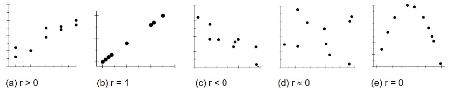
Notice in Figure 2, several scatterplots have been labeled with their correlations.
(a) A scatter plot showing data with a positive correlation, 0 < r < 1, and r would be closer to 1. A best fitting line through the data will have a positive slope.
(b) A scatter plot showing data with perfect linear trend, so a line would exactly pass through each data value and the line would have a positive slope. In this case the correlation coefficient would take on the value 1.
(c) A scatter plot showing data with a negative correlation, -1 < r < 0. A best fitting line through the data will have a negative slope.
(d) A scatter plot showing data with close to zero correlation, r = 0, or only slightly negative. Changing the independent variable does not correspond to any change in the dependent variable.
(e) A scatter plot showing a parabolic trend. In this case there is a strong association between variables but the relationship is not linear. The correlation would be 0.
Correlation is Not Causation
It is always very important to note and remember that just because there is an association between two variables, that does not mean that changing one variable causes changes in another variable. In other words, correlation is not causation. Tyler Vigen produces spurious correlations that are entertaining and the following is provided courtesy of him. It shows that the pounds of margarine consumed is negatively correlated (r = -0.993) with the divorce rate in Maine.
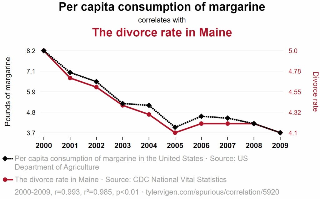
Just because two quantities appear to change together, that does not mean there is a causal relationship between the quantities. There can be another variable correlated with both causing this spurious correlation. A third variable that is correlated with both of the other variables is a lurking variable. Lurking variables can mask a relationship or make a relationship appear greater than it actually is.
Correlation Reminders
- The correlation coefficient r is a measure of the strength and direction of a linear association between two quantitative variables.
- The correlation coefficient is a number between −1 and 1. The closer r is to 1 or −1, the closer the data are to having a perfect linear association.
- The value of r alone cannot tell you if an association between two variables exists. A value of r close to 0 does not mean that there is no association. Before interpreting a correlation coefficient, we must first look at the scatterplot.
- The correlation coefficient measures association, but not causation. A strong correlation between two variables is evidence that there is a statistical relationship between the variables. Only the results of an experiment using random selection can establish a causal connection between two variables.
- A lurking variable affects both explanatory and response variables in a predictable way, and thus creates a statistical relationship between the explanatory and response variable.
Sources
Pahwa, A. (2023, August 4). What is M-Commerce? | The rise of mobile commerce. Feedough. https://www.feedough.com/m-commerce-rise-mobile-commerce/
Mobile Commerce: M-commerce Examples and Trends (2024). (2023, December 22). Shopify. https://www.shopify.com/blog/mobile-commerce
Kennedy, M. (2016, April 20). Lead-Laced Water in Flint: A Step-By-Step look at the makings of a crisis. NPR. https://www.npr.org/sections/thetwo-way/2016/04/20/465545378/lead-laced-water-in-flint-a-step-by-step-look-at-the-makings-of-a-crisis
Vigen, T. (2024, June 23). Spurious Correlations. https://tylervigen.com/spurious-correlations

Feedback/Errata