2.6 Symmetry and Skewness

We gain valuable insight into a population when we look at graphical displays created from the sample information. When we create frequency histograms from sample data, one of the first things we notice is whether the histogram displays symmetry or lacks symmetry.

Symmetry

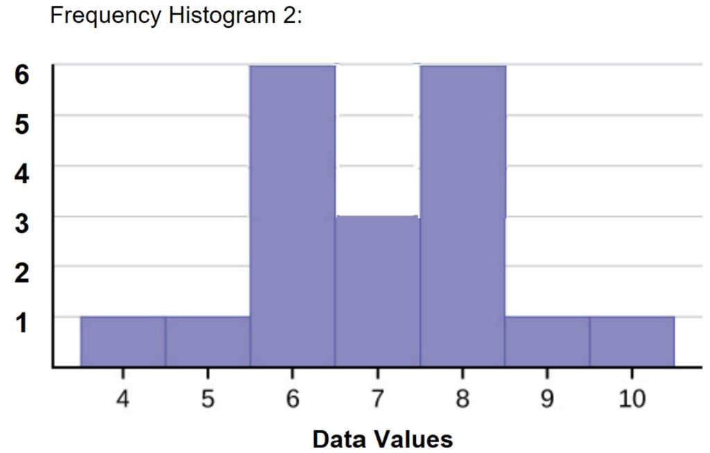
The histograms in Figure 1 and in Figure 2 both display symmetry in the distribution of the data. A distribution is symmetric if a vertical line can be drawn at some point in the histogram such that the shape to the left and the right of the vertical line are mirror images of each other.

Take a look at Frequency Histogram 1. The data used to create the frequency histogram are  4; 5; 6; 6; 6; 7; 7; 7; 7; 7; 7; 8; 8; 8; 9; and 10. For these data, the mean, the median, and the mode are each seven.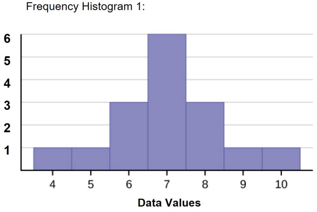

It is worth noting that in a perfectly symmetric distribution, the mean and the median will be the same. Additionally in Frequency Histogram 1, there is a single peak, so there is a single mode. Because this symmetric histogram has one mode, the mode is the same as the mean and median. Keeping this in mind will give you insight into the distribution of data if you are given a mean, median, and mode that are the same value.

Now consider Frequency Histogram 2. The data used to create the frequency histogram are  4; 5; 6; 6; 6; 6; 6; 6; 7; 7; 7; 8; 8; 8; 8; 8; 8; 9; and 10. In a symmetrical distribution that has two modes (bimodal), the two modes can be different from the mean and median. In this case, the modes are 6 and 8, while the mean and median are the same value of 7.

Skewness

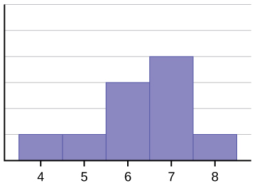
The histogram for the data: 4; 5; 6; 6; 6; 7; 7; 7; 7; 8 is not symmetrical. The right-hand side seems “chopped off” compared to the left side. A distribution of this type is called skewed to the left because it is pulled out to the left. This can also be called negative skewness. You might describe it as having a left-hand “tail”. The mean is 6.3, the median is 6.5, and the mode is 7. Notice that the mean is less than the median, and they are both less than the mode. The mean and the median both reflect the skewing, but the mean reflects it more so.

Frequency Histogram 3:

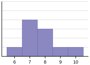
The histogram for the data: 6; 7; 7; 7; 7; 8; 8; 8; 9; 10 is also not symmetrical. It is skewed to the right, or positive skewness. The mean is 7.7, the median is 7.5, and the mode is seven. Of the three statistics, the mean is the largest, while the mode is the smallest. Again, the mean reflects the skewing the most.

Frequency Histogram 4:

To summarize, generally if the distribution of data is skewed to the left, the mean is less than the median, which is often less than the mode. The concentration of the skewed left data is at the upper end of the scale. If the distribution of data is skewed to the right, the mode is often less than the median, which is less than the mean and the concentration of the data is at the lower end of the scale.

Skewness and symmetry become important when we discuss probability distributions in later chapters. We will always want to take a look at the data to see where the data concentrate. We want to see if there is a long tail to the right or the left or whether the data display symmetry.

Here is a video that summarizes how the mean, median and mode can help us describe the skewness of a dataset. Don’t worry about the terms leptokurtic and platykurtic for this course.

Example 1

Discuss the mean, median, and mode for each data set. Connect the values to the symmetry or skewness of the displays.

1.

2.

The Ages Former U.S Presidents Died
4	6 9
5	3 6 7 7 7 8
6	0 0 3 3 4 4 5 6 7 7 7 8
7	0 1 1 2 3 4 7 8 8 9
8	0 1 3 5 8
9	0 0 3 3
Key: 8|0 means 80.

3.

Answers:

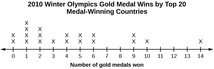
1. The data appear to be skewed to the right, with the bulk of the medals concentrated between 0 metal and 6. We expect to see the mode as the lowest value and the mean pulled higher than the median. For these data the mode is 1, the median is 3.5, and the mean is 8.5.
2. The 39 ages at which former presidents died appear to be fairly symmetric, so there is an expectation that the mean and median will be approximately the same. The median is 68 years while the mean is 70.08. The data set is bimodal, with the ages of 57 and 67 occurring three times each.
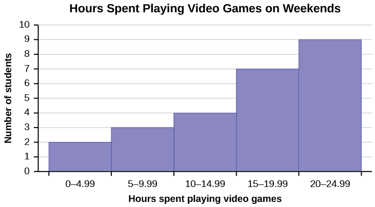
3. For the video game data, we can use the midpoints of each interval in calculations, since we cannot read off the original data values. Notice how skewed left this histogram is. We expect the mean to be pulled to the lower number of hours. The data is more concentrated toward higher values, so the mode is expected to be the largest value. The mean is expected to be the smallest value and the median will be somewhere in between. For these data, the mode is about 22.5 hours (the midpoint of the largest bar). The median is approximately 17.5 hours. The mean is 16.1 hours.