11.3 The F Distribution and F-Test Statistic

Jeff Crabill; Vikki Maurer

11.3 The F Distribution and F-Test Statistic

The distribution used for the analysis of variance hypothesis test is a new one. It is called the F distribution, named after Sir Ronald Fisher, an English statistician. The F distribution is a continuous distribution, with a shape that depends on two sets of degrees of freedom. We will not go into great detail about the F distribution but will present some features.

F Distribution Fun Facts

The F distribution curve is not symmetrical but skewed to the right.
There is a different curve for each set of degrees of freedom in the numerator and denominator. See Figure 1 for two examples.
The F statistic is a fraction and its value greater than or equal to zero.
The F test statistic has two sets of degrees of freedom; one for the numerator and one for the denominator.
As the degrees of freedom for the numerator and for the denominator get larger, the curve approximates the normal.
The F distribution is used when comparing two independent variances.
Other uses for the F distribution include two-way analysis of variance, which is beyond the scope of this text.
The notation for the F distribution is $F \sim F_{\text{df(numerator)},\text{ df(denominator)}}$ .

The curve one the left is a nonsymmetrical F distribution curve skewed to the right, more values in the right tail and the peak is closer to the left. This curve is different from the graph on the right because of the different dfs. The curve on the right shows a nonsymmetrical F distribution curve skewed to the right. This curve is different from the graph on the left because of the different dfs. Because its dfs are larger, it more closely resembles a normal distribution curve. — Figure 1: Two F Distribution Curves with Different Degrees of Freedom

Notation Associated with ANOVA

We will select random samples of size $n$ from each of $k$ independent and normally distributed populations. For each of these populations, the population means are $\mu_1, \mu_2, \cdots, \mu_k$ and each population has the same variance denoted as $\sigma^2$ . This will allow us to conduct the following hypothesis test:

$H_o: \mu_1 = \mu_2 = \cdots = \mu_k$

$H_a:$ At least two of the means are not equal.

Table 1: Generic Notation for One-Factor ANOVA with Equal Sample Sizes
Treatment (Levels of Factor)	Observations in Each of the Treatment Groups				Treatment Means
1	$x_{11}$	$x_{12}$	$\cdots$	$x_{1n}$	$\bar{x}_{1.}$
2	$x_{21}$	$x_{22}$	$\cdots$	$x_{2n}$	$\bar{x}_{2.}$
$\vdots$	$\vdots$	$\vdots$		$\vdots$	$\vdots$
$k$	$x_{k1}$	$x_{k2}$	$\cdots$	$x_{kn}$	$\bar{x}_{k.}$
				Grand Mean =	$\bar{x}_{..}$

F-Test Statistic

When we use the F-test statistic in the context of this hypothesis test, the assumption under the null hypothesis is that the means are all the same. In order to conduct this test, the assumption is made that the variances are the same as well, so each population has a common population variance, $\sigma^2$ . To calculate the F-test statistic, two estimates of the common variance, $\sigma^2$ , are made and compared in a fraction.

$\displaystyle{F = \frac{\text{Variance Between Samples}}{\text{Variance Within Samples}} = \frac{\text{MST}}{\text{MSE}}}$

Variance Between Samples, MST:

The notation “MS” stands for “mean square” so MST represents the variance between the groups.
This is one estimate of $\sigma^2$ , which is the variance of the sample means with the grand mean, multiplied by the common sample size.
This variance is also called the treatment variation or the explained variation.
The differences between the treatment means will affect the size of MST.
The degrees of freedom associated with the numerator is the one less than the number of samples, $k - 1$ .

Variance Within Samples, MSE:

The notation “MS” stands for “mean square”, so MSE represents the variation within a sample.
This is an estimate of $\sigma^2$ , which is the average of the individual sample variances (also known as a pooled variance).
This variance is also called the variation due to error or unexplained variation.
MSE represents the variation within the samples due to chance alone.
Because MSE considers the variation of the values of each group with its own group mean, the differences between groups will not affect it.
The degrees of freedom associated with the denominator is $k(n - 1)$ .

Value of the F-Test Statistic:

When the null hypothesis is true, the two estimates of $\sigma^2$ should be close in value.
If MST is close in value to MSE, then the F-test statistic will take on a value close to one.
Because MST and MSE will always be positive, the F-test statistic will always be positive.
When the null hypothesis is false, MST will be larger than MSE, so the F-test statistic will take on a value greater than one.

Calculations of Sum of Squares and Mean Squares

Although in practice, we will let a statistical package calculate the F-test statistic, to gain insight into the composition of the test statistic, we present the formulas. The one-factor ANOVA is based on a comparison of two independent estimates of the common population variance, $\sigma^2$ . This is done by splitting up the total variation in the data into two parts.

Sum of Squares Total = Sum of Squares Treatment (SST) + Sum of Squares Error (SSE)

$\sum_{i=1}^k\sum_{j=1}^n\left(x_{ij}-\bar{x}_{..}\right)^2=n\sum_{i=1}^k\left(\bar{x}_{i.}-\bar{x}_{..}\right)^2+\sum_{i=1}^k\sum_{j=1}^n\left(x_{ij}-\bar{x}_{i.}\right)^2$

Data are typically put into a table for easy viewing. One-Way ANOVA results are often displayed as shown in Table 2.

Table 2: Statistical Package Typical ANOVA Output
Source of Variation	DF	Sum of Squares	Mean Square	F Value	P-Value
Factor or Treatment (Variation Between Groups)	$k-1$	SST	MST = SST/( $k-1$ )	F = MST/MSE	P(F $\geq$ MST/MSE)
Residual or Error (Variation Within Groups	$k(n-1)$	SSE	MSE = SSE/( $k(n-1)$ )
Total Variation	$kn-1$	Sum of Squares Total

Example 1 – Fever Reducing Drugs

A researcher would like to compare the effect of different fever reducing treatments on body temperature. Thirty-five patients were randomly assigned into five treatment groups, so there were seven patients in each group. The patients’ temperatures were taken two hours after receiving the treatment, and these are given in Table 1. Use a one-way ANOVA to test the claim that there is no difference in mean body temperature among each of the five treatment groups using a 1% significance level. Assume the independent samples were drawn from normal populations with equal variances.

Table 3: Temperatures of 35 People Who Received a Treatment
Placebo	Aspirin	Anacin	Tylenol	Bufferin
98.3	96.0	97.2	95.1	96.1
98.7	96.6	97.4	95.7	96.5
98.1	95.3	96.9	94.4	95.4
99.9	98.1	97.8	97.2	98.2
96.2	94.6	94.7	93.7	94.5
98.6	96.6	97.0	95.7	96.5
98.3	96.2	96.8	95.3	96.2

Solution:

In this experiment, there is one factor, the fever-reducing treatment. The five levels of the factor are the individual drugs and placebo. Each of the five groups has a sample size of seven. The alternate hypothesis will state that at least two of the mean body temperatures are not equal, so the null hypothesis will state that all the mean body temperatures are the same.

$H_o: \mu_1 = \mu_2 = \cdots = \mu_k$

$H_a:$ At least two of the means are not equal.

Using a statistical program, the ANOVA table is provided in Table 4.

Table 4: ANOVA Output for Temperature
Source of Variation	DF	Sum of Squares	Mean Square	F Value	P-Value
Factor or Treatment (Variation Between Groups)	4	34.2131	8.55329	F = 7.14589	0.000363
Residual or Error (Variation Within Groups	30	35.9086	1.19695
Total Variation	35	Sum of Squares Total

When the null hypothesis is true, the F-test statistic should be close to 1. When the null hypothesis is false, there is a difference in the population means, so the F-test statistic should be greater than 1. In this case F = 7.14589. This F-test statistic indicates that the variance between the samples is about 7 times as large as the variance within the samples.

Under the null hypothesis, the F-test statistic has an F distribution with 4 and 30 degrees of freedom. The p-value is calculated as 0.000363 and is the area shown in Figure 2.

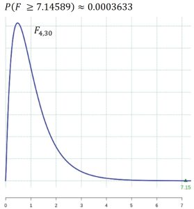
Graph of F distribution with 4 and 30 degrees of freedom showing the area shaded to the right of 7.14589 giving a p-value of 0.0003633. — Figure 2: P-Value Graph

Because the p-value is much less that the 1% level of significance, we strongly reject the null hypothesis and conclude at least one of the treatments yields a mean body temperature that is different from the other treatments.

Sources

Example 1 is adapted from Statway College Module 5 by Carnegie Math Pathways is licensed under CC BY NC 4.0.

License

Icon for the Creative Commons Attribution 4.0 International License

Introduction to Statistics for Engineers Copyright © by Vikki Maurer & Jeff Crabill & Linn-Benton Community College is licensed under a Creative Commons Attribution 4.0 International License, except where otherwise noted.

Feedback/Errata

Comments are closed.