6.3 The Uniform Distribution
The uniform distribution is a continuous probability distribution and is concerned with events that are equally likely to occur within a specific range. Many computer algorithms generate pseudo-random numbers uniformly distributed between 0 and 1. This uniform distribution ensures that each value within the range has an equal probability of being generated. Because every value on an interval occurs with equal probability, the probability density function, ![]() is constant. It is often referred as the rectangular distribution because the graph of the pdf has the form of a rectangle.
is constant. It is often referred as the rectangular distribution because the graph of the pdf has the form of a rectangle.
The probability ![]() may be found by computing the area under
may be found by computing the area under ![]() between a and b, as shown in Figure 1. Since the corresponding area is a rectangle, the area may be found simply by multiplying the width and the height. Because the area represents the total probability, the length of the rectangle multiplied by the height must be 1. Thus,
between a and b, as shown in Figure 1. Since the corresponding area is a rectangle, the area may be found simply by multiplying the width and the height. Because the area represents the total probability, the length of the rectangle multiplied by the height must be 1. Thus, ![]()
Hence it is clear that the PDF for the uniform distribution is ![]() .
.

Facts about the Uniform Distribution
Once you have established that a continuous random variable X has a uniform distribution on the interval ![]() , then we know the following:
, then we know the following:
- We use the notation

- The PDF is

- The mean of the uniform distribution is

- The standard deviation of the uniform distribution is
 .
.
The mean and standard deviations can be derived using the integral definitions presented in section 6.2.
Example 1 – Random Number Generator
A random number generator generates numbers between (and including) 0 and 20, so each number has an equal chance of being selected. If X = a randomly generated number from 0 to 20, then ![]() .
.
- Create the PDF.
- Calculate the probability of selecting a number between 0 and 2.
- Calculate the mean and standard deviation.
Solutions:
- The PDF is a constant function,
 over the domain
  Note the total area is 1.
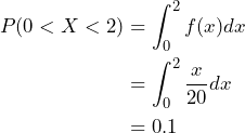
 - To compute the probability to selecting a number between 0 and 2, we compute
 . (Note that here we could just as well do a simple geometric calculation.)

- The mean of the random variable is
 , and the standard deviation is
 , using the formulas above.
Example 2 – Bus Waiting Time
The amount of time, in minutes, that a person must wait for a bus is uniformly distributed between zero and 15 minutes, inclusive.
- What is the probability that a person waits fewer than 12.5 minutes?
- On the average, how long must a person wait? Find the mean, μ, and the standard deviation, σ.
- Ninety percent of the time, the time a person must wait falls below what value? This asks for the 90th percentile.
Solutions:
First, we establish the probability distribution of the random variable. In this case X measures the time that a person waits for a bus. In addition, we know that ![]() The PDF is
The PDF is ![]()
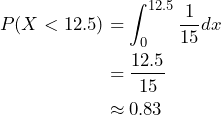
- The probability that a person waits fewer than 12.5 minutes is
 , and is shown in the shaded region in the diagram. To compute, we either set up an integral or we use geometry to find the area.
.Approximately 83% of the time a person will wait fewer than 12.5 minutes for the bus.
- To find the average time a person will wait, we compute the mean or the expected value of the random variable. Here,
 , or alternately,
  . Likewise,
  On average, a person must wait 7.5 minutes with a standard deviation of 4.33 minutes.
 - To find the 90th percentile, we’ll use geometry! We must find the value of
 that marks the boundary between the lower 90% and upper 10% of the data. (Geometry is the most useful tool when working with the uniform distribution.)
Since the shaded area is the probability we’re looking for, we know that ![]() .
.
Thus ![]() and
and ![]() .
.
So the 90th percentile is 13.5 minutes. Ninety percent of the time, a random person will wait at most 13.5 minutes for the bus.


Feedback/Errata