10.2 Inference for the Difference Between Independent Groups

Jeff Crabill; Vikki Maurer

10.2 Inference for the Difference Between Independent Groups

Conducting a hypothesis test for two independent groups is a fundamental statistical process that allows us to determine whether there is a significant difference between their means. This type of test is essential in various fields, including engineering, science, and social studies. Consider several scenarios:

Comparing Performance of Two Designs: Engineers often need to compare the performance of two different designs or prototypes. For example, they might compare the efficiency of two different engine models to determine if there is a significant difference in their fuel consumption.
Testing New Materials: When introducing a new material, engineers might compare its performance against the current standard material. For example, testing the tensile strength of a new alloy compared to the existing one.
Supplier Comparison: When sourcing components from two different suppliers, engineers might to determine if there is a significant difference in the quality or performance of components from each supplier.

In this section we will consider the situation in which the populations from which the samples are drawn are normal, the variances are unknown, and the sample sizes are not large. In this situation previously, we have relied on the Student’s t-distribution, and we will again. However, there is a bit more to consider. We must keep in mind that the difference between the two samples depends on both the means and the standard deviations. Very different means can occur by chance if there is great variation among the individual samples. Thus, variation is an important consideration when working with two independent groups, and depending on what we can assume, will lead to two different versions of a hypothesis test.

Tests for Comparing Two Independent Groups

As we begin the process of comparing two independent groups, our notation will need to differentiate between the groups. Consider two independent samples in Figure 1. We will use subscripts to denote the parameters and statistics that belong to each population and sample.

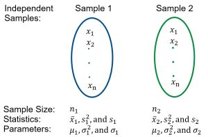
Visual depiction of two samples showing the use of subscripts for each statistic and parameter to indicate into which sample or population each belongs. — Figure 1: Independent Samples from Two Populations

For the two samples we might wonder if the means of the two populations are the different, $\mu_1 \neq \mu_2$ , or if one population has a greater mean, $\mu_1 > \mu_2$ or $\mu_1 < \mu_2$ . The corresponding null hypotheses will state one of the following:

$H_o: \mu_1 = \mu_2$ or equivalently $H_o: \mu_1 - \mu_2 = 0$

$H_o: \mu_1 \leq \mu_2$ or equivalently $H_o: \mu_1 - \mu_2 \leq 0$

$H_o: \mu_1 \geq \mu_2$ or equivalently $H_o: \mu_1 - \mu_2 \geq 0$

We can also test whether the difference between the means is some specified difference, $d_o$ , so the difference does not always have to be set to zero. The point estimate of the difference of two population means, $H_o: \mu_1 - \mu_2$ , is the difference in the sample means, $\bar{x}_1 - \bar{x}_2$ . At this point we typically present the test statistic and the distribution of the test statistic. Because we are dealing with two different samples, and we have two sample variances to consider, how they are combined to create the variance and standard deviation of the sampling distribution matters.

Exact or Pooled Test: If the variances from the two independent populations are approximately equivalent, and this is something that would need to be checked into before moving forward, then an exact t-test can be performed because the distribution of the sample mean difference, $\bar{x}_1 - \bar{x}_2$ would have a Student’s t-distribution. In this case the variance of the sample statistic would be created through a pooling of the sample variances. Because of this, the exact t-test is often called a “pooled” t-test. The pooling creates a weighted average of the individual sample variances, and the pooled variance is an unbiased estimator of the common population variance.
Approximate Test: If we cannot assume that the variances from the two independent samples are approximately equivalent, then there can be no pooling of the sample variances, and the t-test statistic will be only approximately distributed as the Student’s t-distribution. The approximate test will be a more conservative test than the exact test, and would require larger differences between the sample means to produce a significant result.

The two versions of the test for the difference between independent groups are presented next. The formulas for the pooled variance and degrees of freedom are presented for completeness, however, we will let a statistical package run the actual calculations.

Pooled Two-Sample T-Test

When two independent random samples, each from normal populations, have equal variances but they are not known, then the underlying distribution of $\bar{x}_1 - \bar{x}_2$ is the exact Student’s t-distribution. In order to specify the standard error (standard deviation of the sampling distribution), we use a weighted average and pool the sample variances to create a pooled sample standard deviation, $s_p$ .

$\displaystyle{s_p = \sqrt{\frac{(n_1 - 1)s_1^2+(n_2 - 1)s_2^2}{n_1 + n_2 - 2}}}$

For hypothesis tests involving: $H_o: \mu_1 - \mu_2 = d_o$ , $H_o: \mu_1 - \mu_2 \leq d_o$ , $H_o: \mu_1 - \mu_2 \geq d_o$ ,

We assume $H_o$ is true, so the null distribution of the sample mean difference is an exact Student’s t-distribution: $\bar{x}_1 - \bar{x}_2 \sim t_v(\mu_1 - \mu_2, s_p\sqrt{\frac{1}{n_1} + \frac{1}{n_2}}\bigg)$ with degrees of freedom, $v = n_1 + n_2 - 2$ .

The test statistic (t-score) is $\displaystyle{t =\frac{(\bar{x}_1 - \bar{x}_2) - d_o}{s_p\sqrt{\frac{1}{n_1} + \frac{1}{n_2 }}}}$ .

Probability associated with the test statistic can be found from the Student’s t-distribution with $v$ degrees of freedom. Equivalently the p-value can be found directly using the null distribution directly.

If $H_a: \mu_1 - \mu_2 \neq d_o$ , calculate the p-value as the sum of the areas in the tails cut of by $-t$ and $t$ .

If $H_a: \mu_1 - \mu_2 > d_o$ , calculate the p-value as the sum of the area to the right of the test statistic, $t$ .

If $H_a: \mu_1 - \mu_2 < d_o$ , calculate the p-value as the sum of the area to the left of the test statistic, $t$ .

In order to use the pooled two-sample t-test, the variances of the two samples are pooled together. This provides an estimate of the population variance. It is important to note that this test will not perform well if the population variances are actually not equal, and of course, there is never a way to know for sure. There are suggestions that the unequal variance two-sample t-test is preferred.

Approximate Two-Sample T-Test (Whelch’s Test)

When two independent random samples, each from normal populations, have unknown and unequal variances, then the underlying distribution of $\bar{x}_1 - \bar{x}_2$ is an approximate Student’s t-distribution.

For hypothesis tests involving: $H_o: \mu_1 - \mu_2 = d_o$ , $H_o: \mu_1 - \mu_2 \leq d_o$ , $H_o: \mu_1 - \mu_2 \geq d_o$ ,

We assume $H_o$ is true, so the null distribution of the sample mean difference is an approximate Student’s t-distribution: $\bar{x}_1 - \bar{x}_2 \sim t_v\bigg(\mu_1 - \mu_2, \sqrt{\frac{s_{1}^2}{n_1} + \frac{s_{2}^2}{n_2}}\bigg)$ with degrees of freedom, $v$ calculated as:

$\displaystyle{v =\frac{(\sfrac{s_1^2}{n_1}+ \sfrac{s_2^2}{n_2})^2}{\sfrac{(\sfrac{s_1^2}{n_1})^2}{(n_1-1)}+\sfrac{(\sfrac{s_2^2}{n_2})^2}{(n_2-1)}}}$

The test statistic (t-score) is $\displaystyle{t =\frac{(\bar{x}_1 - \bar{x}_2) - d_o}{\sqrt{\frac{s_1^2}{n_1} + \frac{s_2^2}{n_2}}}}$ .

Probability associated with the test statistic can be found from the Student’s t-distribution with $v$ degrees of freedom. Equivalently the p-value can be found directly using the null distribution directly.

If $H_a: \mu_1 - \mu_2 \neq d_o$ , calculate the p-value as the sum of the areas in the tails cut of by $-t$ and $t$ .

If $H_a: \mu_1 - \mu_2 > d_o$ , calculate the p-value as the sum of the area to the right of the test statistic, $t$ .

If $H_a: \mu_1 - \mu_2 < d_o$ , calculate the p-value as the sum of the area to the left of the test statistic, $t$ .

Example 1 – Driving Behaviors

A phycologist was interested in exploring whether or not female and male college students have different driving behaviors. A particular focus of the experiment was to focus on the fastest speed driven by an individual. A survey of 34 randomly selected male college students and 29 randomly selected female college students was conducted. See Table 1 for the summary statistics. Is there evidence to conclude that the mean fastest speed driven by male college students different from the mean fastest speed driven by female college students? Use a 5% level of significance. Assume that normal probability plots of the samples provided support to assume the populations are normally distributed.

Table 1: Summary Statistics
Sample 1: Males	Sample 2: Females
$n_1 = 34$	$n_2 = 29$
$\bar{x}_1 = 105.5$	$\bar{x}_2 = 90.9$
$s_1 = 20.1$	$s_2 = 17.8$

Solution:

The research question alternate hypothesis states that the mean fastest speeds are different, so the null hypothesis will state that the speeds are the same.
$H_o: \mu_1 - \mu_2 = 0$
$H_a: \mu_1 - \mu_2 \neq 0$
These two samples came from independent populations, since random sampling was conducted. Note that the sample standard deviations are close in value, so we will assume the population standard deviations are equal and use the pooled t-test to test the claim:
$\displaystyle{s_p = \sqrt{\frac{(34 - 1)20.1^2+(29 - 1)17.8^2}{34 + 29 - 2}}\approx 19.0787}$
Under these conditions the sampling distribution is the Student’s t-distribution with $v = 34 + 29 - 2 = 61$ degrees of freedom.
Therefore, $\bar{x}_1 - \bar{x}_2 \sim t_{61}\bigg(0, s_p\sqrt{\frac{1}{34} + \frac{1}{29}}\bigg)$ and the t-test statistic will be used.
The test statistic is $\displaystyle{t =\frac{(105.5 - 90.9) - 0}{19.0787\sqrt{\frac{1}{34} + \frac{1}{29 }}}\approx 3.027}$ .
The p-value is the probability of observing a sample mean as extreme as we did under the assumption that the null hypothesis is true. Because this is a two-tailed test, calculate the probability as $P(t < -3.027) + P(t > 3.027) \approx 0.0036$ . See Figure 2.

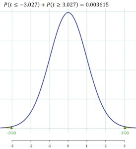
Figure 2: P-value Shaded
Assuming the null hypothesis is true and there is no difference, there is a 0.36% chance of observing a sample as extreme as we did, therefore, there is evidence to reject the null hypothesis at the 5% significance level. We conclude that the evidence suggests the mean fastest speed driven by male college students is different from the mean fastest speed driven by female college students.

Example 2 – Heart Attack in Sheep

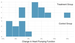
A researcher is wondering if treatment using embryonic stem cells in sheep help improve heart function following a heart attack. Sheep were randomly selected and assigned to two groups: the treatment group $T$ and the control group $C$ . The study measured the change in the sheep’s heart pumping capacity, where a positive value indicates increased pumping capacity, suggesting stronger recovery. Figure 3 contains two histograms of the data and Table 2 contains the summary statistics from the study.

Table 2: Sheep Study Summary Statistics
Treatment Group	Control Group
$\bar{x}_T = 3.50$	$\bar{x}_C = -4.33$
$s_T = 5.17$	$s_C = 2.76$
$n_T = 9$	$n_C = 9$

Two histograms of data from the sheep study. Both show no outliers. — Figure 3: Histograms of Sheep Data

Is there evidence to conclude that the mean change in the treatment group is greater than the mean change in the control group? Use a 5% level of significance.

Solution:

The alternate hypothesis states that the mean of the treatment group is greater than the mean of the control group, so the null hypothesis will state that the means are at most the same.
$H_o: \mu_T - \mu_C \leq 0$
$H_a: \mu_T - \mu_C > 0$
These two samples came from independent populations, since random sampling was conducted. Note from Figure 3 that the histograms of the sample data do not show outliers and are reasonably symmetric, so the assumption that both samples came from normal populations is met. Also note that the sample standard deviations are not close in value, so we will assume the population standard deviations are not equal and use the independent t-test to test the claim.
Under these conditions the sampling distribution is the approximate Student’s t-distribution with
$\displaystyle{v =\frac{(\sfrac{5.17^2}{9}+ \sfrac{2.76^2}{9})^2}{\sfrac{(\sfrac{5.17^2}{9})^2}{8}+\sfrac{(\sfrac{2.76^2}{9})^2}{8}} \approx 12.2174}$ degrees of freedom.
Therefore, under the null hypothesis, $\bar{x}_1 - \bar{x}_2 \sim t_{12.217}\bigg(0, \sqrt{\frac{5.17^2}{9} + \frac{2.76^2}{9}}\bigg)$ and the t-test statistic will be used.
The test statistic is $\displaystyle{t =\frac{(3.50 - (-4.33) - 0}{\sqrt{\frac{5.17^2}{9} + \frac{2.76^2}{9 }}} \approx 4.0081}$ .
The p-value is the probability of observing a sample mean as extreme as we did under the assumption that the null hypothesis is true. Because this is a right-tailed test, calculate the probability as $P(t > 4.0081) \approx 0.0008$ . See Figure 3.

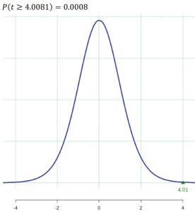
Figure 3: P-value
Assuming the null hypothesis is true, there is a 0.08% chance of observing a sample as extreme as we did, therefore, there is strong evidence to reject the null hypothesis at the 5% significance level. We conclude that the evidence suggests the the mean change in the treatment group is greater than the mean change in the control group.

Sources

B. L. Welch, The Generalization of “Student’s” Problem When Several Different Population Variances are Involved, Biometrika, Volume 34, Issue 1-2, January 1947, Pages 28–35, https://doi.org/10.1093/biomet/34.1-2.28

License

Icon for the Creative Commons Attribution 4.0 International License

Introduction to Statistics for Engineers Copyright © by Vikki Maurer & Jeff Crabill & Linn-Benton Community College is licensed under a Creative Commons Attribution 4.0 International License, except where otherwise noted.

Feedback/Errata

Comments are closed.