6.6 Normal Distribution Probabilities

Jeff Crabill; Vikki Maurer

6.6 Normal Distribution Probabilities

In this section, we’ll be computing probabilities of normally distributed random variables. Just like with the uniform distribution in a previous section, once we establish that a random variable has a given distribution, we can use the PDF to compute probabilities using an integral. In the case of a normally distributed random variable,

$P(a < X < b) = \displaystyle\int_a^b \frac{1}{\sigma\sqrt{2\pi}} e^{ -\frac{1}{2} \left( \frac{x-\mu}{\sigma}\right)^2 }dx$

would be the probability a normally distributed random variable takes on values between $x = a$ and $x = b$ .

No Antiderivative

As a student of calculus, you may be tempted to start by looking for an antiderivative, however this particular integral has no closed-form antiderivative, so the numerical integration done by computers is the best way to compute probabilities in this case.

You should be using some form of technology at this point to compute probabilities.

Relating the Shaded Area to Probability

Always keep the relationship between area under the PDF and probability in the front of your mind when you are computing probabilities. Some technology tools will compute $P(X < x)$ only, while others will give you the option to compute other probabilities. Make sure you know how to use your chosen technology tool before you rely on it!

Figure 1 shows the area $P(X < x)$ shaded in purple. You can very easily find $P(X > x)$ by computing $1 - P(X < x)$ .

This is a normal distribution curve. A value, x, is labeled on the horizontal axis, X. A vertical line extends from point x to the curve, and the area under the curve to the left of x is shaded. The area of this shaded section represents the probability that a value of the variable is less than x. — Figure 1: P(X < x)

No Area at a Point

When working with a continuous probability distribution, there is no distinction between $P(X < x)$ and $P(X \leq x)$ . The values are equal because the inclusion of the single value $x$ does not change the value of the integral. Remember there is no area associated with a single x-value.

Calculations of Probabilities Using Technology

Probabilities related to the normal distribution are calculated using technology. Make sure to familiarize yourself with the tool of your choice! Popular choices include the following, in no particular order:

Desmos
Spreadsheets (excel or google sheets)
- “norm.dist” command gets you probabilities
- “norm.inv” command gets you scores
Rguroo
Various online calculators on the internet

There is no “best” or “worst” tool. Choose a tool that works for you and is available!

Example 1: Retirement Age

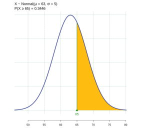
According to a 2024 Forbes Magazine article, the average retirement age in Oregon is 63. Assume the age of retirement is normally distributed with a mean of 63 and a standard deviation of 5. Find each of the following using technology and create a normal distribution to demonstrate the result.

Find the probability that a randomly selected Oregonian retires at age 65 or above.
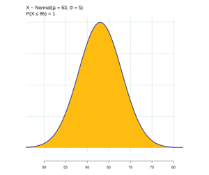
Find the probability that a randomly selected Oregonian retires at less than 85 years old.
Find the 90th percentile (that is, find the value k that has 90% of the ages below k and 10% of the ages above k).

Solution:

Let X = the age at retirement in Oregon, then $X \sim N(63, 5)$ .

(1) The probability an Oregonian retires at age 65 or later is calculated as $P(x > 65)$ is 0.3446. About 34% of Oregonians at age 65 or above.
bell curve centered at 63 with the area shaded in from 65 to infinity

(2) The probability an Oregonian retires by age 85 is calculated as $P(x < 85)$ is 1. About 100% of Oregonians retire by age 85.

normal curve centered at 63 that is entirely filled in with area at score 85 and below (3) We are asked to find the 90th percentile retirement age. Draw the shaded area and notice that the age is unknown. Use technology to find the age that divides the lower 90% and the upper 10% of the data. The age at the 90th percentile is 69.4 years, so approximately 90% of Oregonians retire by age 69.4 years. 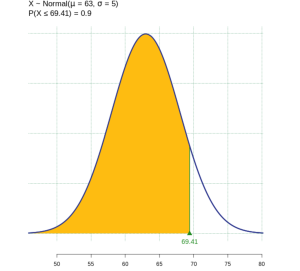a normal curve with the lower 90 percent of the area shaded and an indication that the boundary occurs at score 65.4

Example 2: Equipment Recalibration

An open-source learning management system has a weekly down-time mean of 2 hours, with a standard deviation of 0.5 hours. Assuming down times are normally distributed find the following and draw the corresponding normal distribution diagram.

The probability a random week will experience a down time of 1.8 and 2.75 hours.
Find the 25th percentile of down times.

Solutions:

If X is the down time for an open-source learning management system, we assume $X \sim N(2, 0.5).$

Find $P(1.8 < X < 2.75)$ using technology of your choice. The center of the normal distribution is $\mu = 2$ and the corresponding distribution is sketched with the probability shaded. The probability of a down time of 1.8 to 2.75 hours is 0.5886. In a random week, there is about a 59% chance of a down time between 1.8 and 2.75 hours.
The 25th percentile is the value of the random variable for which 25% of the area is below, as sketched. For this distribution find k, so that $P(x < k) = 0.25$ . In this case, k = 1.66. Thus, approximately 25% of down times in a week will be less than 1.66 hours.

Sources

Tretina, K. (2024, January 26). The average age of retirement in the U.S. Forbes Advisor. https://www.forbes.com/advisor/retirement/average-retirement-age/

License

Icon for the Creative Commons Attribution 4.0 International License

Introduction to Statistics for Engineers Copyright © by Vikki Maurer & Jeff Crabill & Linn-Benton Community College is licensed under a Creative Commons Attribution 4.0 International License, except where otherwise noted.

Share This Book

Feedback/Errata

Comments are closed.