
3.4 Preparing to Print
Learning Objectives
- Locate and fix formatting consistency errors.
- Apply new formatting techniques.
- Use Print Titles to repeat rows and columns on each page of a multiple page worksheet.
- Control where page breaks occur in a multiple page worksheet.
In this section, we will review a worksheet for formatting consistency, as well as learn two new formatting techniques. This worksheet currently prints on four pages, so we will learn new page setup options to control how these pages print. A new data file will be used for this section.
Reviewing Formatting for Consistency
Open the “CH3-Gradebook and Parks” workbook if it isn’t already open.
Click on the “Park Size” sheet tab within your “CH3-Gradebook and Parks” workbook ![]() .
.
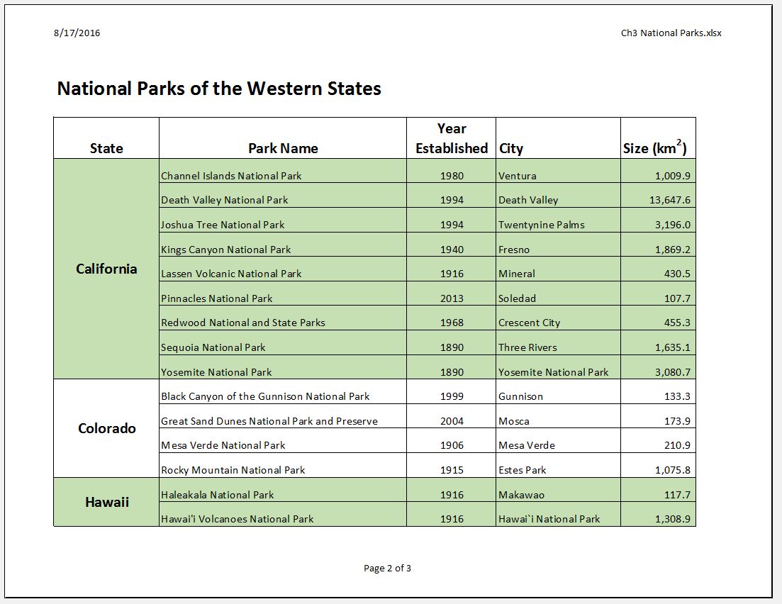
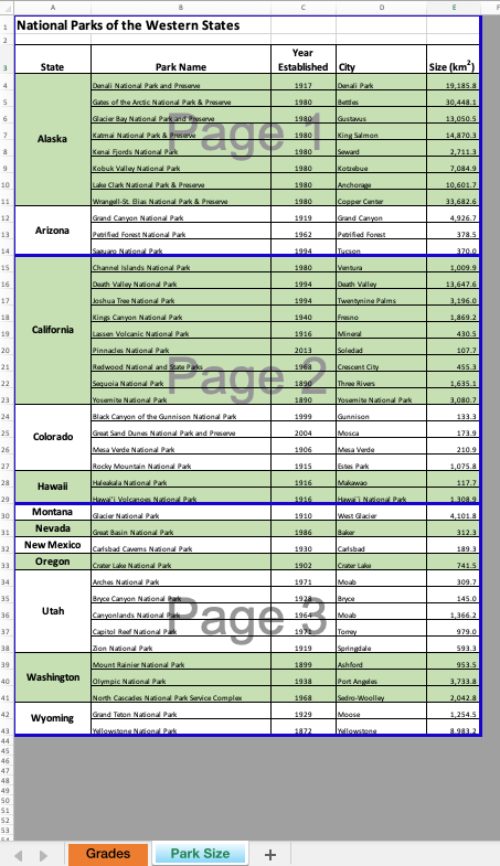
You have been given a spreadsheet with data about the national parks in the western United States. Your coworker formatted the workbook and has asked you to review it for consistency. You also need to prepare it for printing. Figure 3.26 shows how the second page of the finished worksheet will appear in Print Preview.
Reviewing Formatting for Inconsistencies
The first thing you are going to do is review the worksheet for formatting inconsistencies.
- Scroll through the worksheet and locate the following formatting errors:
- The formatting of the Utah label does not match the other states.
- The Year Established values for Hawaii are not center aligned like the other years.
- The cells for the Nevada data should have the same green fill color as the other alternating states.
- The number of digits after the decimal place for the Size values is inconsistent. Also, these values should be formatted with Comma style to make them easier to read.
- To fix these errors, complete the following steps:
- Merge & Center A34:A38. Change the font size to 16 and apply Bold format.
- Center align C28:C29.
- Apply the green fill color to A31:E31 (be sure to match the green fill color of the other states).
- Select E4:E43 and apply Comma Style. Use Increase Decimal and/or Decrease Decimal until one digit appears after the decimal place for all values.
- While you’re fixing errors, proofread the sheet and correct any typos.
- Finally, let’s add color to the two sheet tabs. The use of colored tabs assists in navigating between sheet tabs.
- Right-click the “Park Size” sheet tab (
 Mac users hold down Ctrl key and click the sheet tab)
 - Point to Tab Color and choose a “blue” color.
- Now right-click the “Grades” sheet tab, point to Tab Color and choose an “orange” color. That’s it!
- Right-click the “Park Size” sheet tab (
Fine-tuning Formatting
Now that you have fixed the inconsistencies in the formatting, you decide to apply some formatting techniques to make the worksheet look even better. You are going to start by vertically aligning the names of the states within the cells.
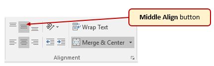
- Select A4:A43 (the cells with the state labels).
- Click the Home tab on the ribbon.
- In the Alignment group, click the Middle Align button (see Figure 3.26). Notice that the names of the states are now centered between the top and bottom borders of the cells.
The next new formatting skill is to change the label in E3 from Size (km2) to Size (km2) with the 2 after km formatted with superscript.
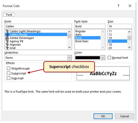
- Double-click on cell E3 to enter Edit mode
- Select just the 2 (be careful not to select anything else).
- On the ribbon (Home tab) click the dialog box launcher arrow in the Font group.
Mac Users: there is no dialog box launcher for Excel for Mac. Instead, choose Format from the Menu Bar, click Cells: 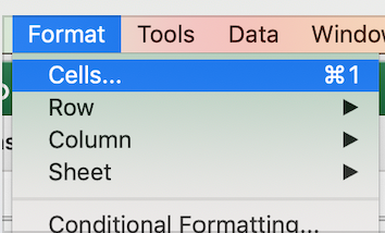 then continue with Steps 4 and 5
 - In the Effects section of the Format Cells dialog box, check the box for Superscript (see Figure 3-27). Click OK.
- Save the CH3 Gradebook and Parks file.
Repeating Column (and Row) Labels
Now that you have fixed the cell and text formatting, you are ready to review the worksheet in Print Preview. You will notice that the worksheet is printing on multiple pages, and you cannot tell what each column of data represents on some of the pages.
- With the CH3-Gradebook and Parks file still open, and the Parks tab selected, go to Backstage View by clicking the File tab on the ribbon. Select Print from the menu.
Mac Users: choose File from the Menu Bar, and then choose Print - Click through each of the pages. The worksheet is currently printing on four pages ( Mac users may only see three pages but that is ok), with the City and Sizes columns printing on separate pages from the rest of the data.
- Change the Orientation from Portrait to Landscape. This fits all of the columns on one page. All of the columns are now on the same page, but the second and third pages have no column labels to identify what information is in each column. You are going to use Print Titles to repeat the first three rows of the worksheet on each of the printed pages. To set Print Titles you need to exit Print Preview.
- Exit Backstage View then click the Page Layout tab on the ribbon.
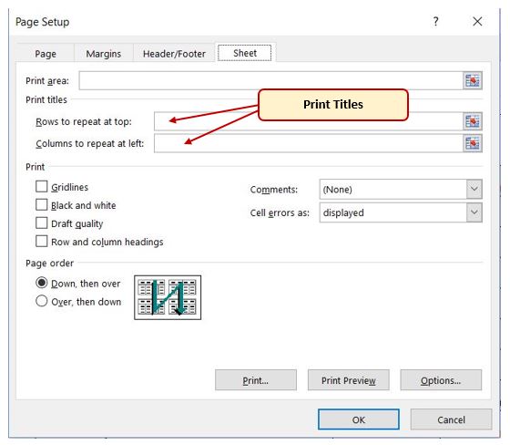
- Click the Print Titles button in the Page Setup group on the ribbon. The dialog box shown in Figure 3.28 should appear.
- Click the Sheet tab if necessary.

- Click in the Rows to repeat at top: box. Be sure your insertion point is blinking in that box before moving on to the next step.
- In the worksheet, select Rows 1 through 3. The text $1:$3 should now appear in the Rows to repeat at top: box.
- Click OK.
You will not see a change to the worksheet in Normal view, so you will need to return to Print Preview. While looking in Print Preview, you will notice that the pages are breaking in inconvenient places.
- Go to Print Preview and look at each of the pages. Notice that the first three rows are now repeated at the top of each page.
- Exit Backstage View.
Skill Refresher
Creating Print Titles
- Open the Page Setup dialog box and click the Sheet tab.
- Click in the Rows to repeat at top: box or the Columns to repeat at left: box.
- Click in the worksheet and select the row(s) or column(s) that you want to repeat on each page.
Inserting Page Breaks
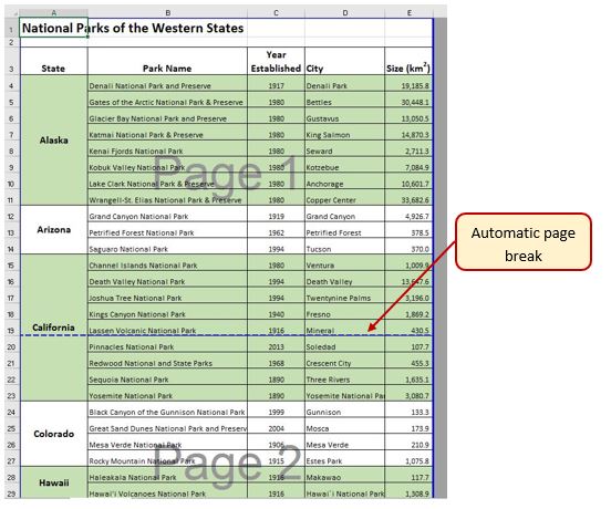
Notice that the data for California is split between the first and second pages. You want all of the data for each state to be together on the same page, so you need to control the page breaks. You are going to start by inserting a page break before the California data to force it to start on the second page, then you will move the page break for the third page if needed. To make these changes you are going to work in Page Break Preview.
- Click the View tab on the ribbon then click Page Break Preview in the Workbook Views Group. Your screen should look similar to Figure 3.29.
![]() Mac Users: in the next paragraph below, the location of the automatic page breaks may be in different locations. That’s ok.
Mac Users: in the next paragraph below, the location of the automatic page breaks may be in different locations. That’s ok.
In Page Break Preview, automatic page breaks are displayed as dotted blue lines. Notice the dotted blue lines after rows 13 and 28. These lines indicate where Excel will start a new page. For this worksheet, you want the first page to break before the California data, so you are going to insert a manual page break.
- Select cell A15. When inserting a page break, you select the cell below where you want the page break to appear.
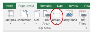
- Click the Page Layout tab on the ribbon.
- Click the Breaks button in the Page Setup group (see Figure 3.30).
- Select Insert Page Break from the menu. There is now a solid blue line after row 14, which indicates a manual page break that was inserted.
- Go to Print Preview. Notice that the California data now starts on the second page.
While looking at each page in Print Preview you decide that the third page should start with Montana. To make this change you are going to move the automatic page break that appears after Nevada.
- Exit Backstage View. Switch back to Page Break Preview if needed.
- Locate the next dotted blue line (automatic page break).
- Put your pointer over the dotted blue line and it will switch to a vertical double-headed arrow. Click on the dotted blue line and drag it above Montana.
- Release the mouse button when the line is above row 30 (above Montana). The line will now be a solid blue line, indicating a manual page break.
- Go to Print Preview. The Montana data now appears at the top of the third page.
While evaluating the pages in Print Preview you decide that there is too much white space at the bottom of the pages. To fix this, you are going to center the contents vertically on the pages.
- Click the Page Setup link at the bottom of the Settings section of Backstage View to open the Page Setup dialog box.
Mac Users: there is no “Page Setup link” in Print Preview for Excel for Mac. Click the Margins list arrow instead, and choose “Manage Custom Margins” then continue with the steps below. 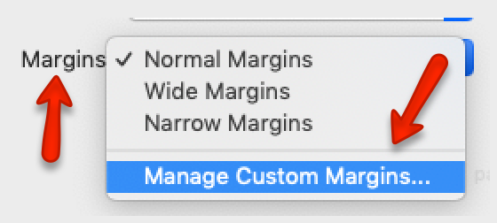
- Click on the Margins tab.
- In the Center on page section, check the box for Vertically then click OK.
- Review each page in Print Preview to see the changes. Exit Backstage View.
Creating a Header and Footer using Page Layout View
Now that the worksheet is printing on three pages, with page breaks in appropriate places, you are ready to add a header with the current date and filename. You will also add a footer with the page number and the total number of pages that will appear as Page 1 of 3. You are going to edit the header and footer in Page Layout View.
- Click the View tab on the ribbon and click the Page Layout button in the Workbook Views group.
- The white space at the top of the worksheet should say Add header. Place the mouse pointer over the left section of the Header and click to activate that section.
Mac Users should make sure the mouse pointer turns into a small page icon  then click in the left section of the Header
 - Click the Header & Footer Tools Design tab on the ribbon.
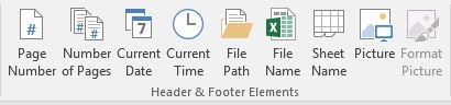
- Click the Current Date button in the Header & Footer Elements group (see Figure 3.31). Inserting the date this way will insert a field that will update every time the workbook is opened.
- Click in the right section of the Header. Click the Filename button in the Header & Footer Elements group (see Figure 3.31). Inserting the filename this way will insert a field that will update if the filename is changed.
- Click the Go to Footer button in the Navigation group of commands.
- In the center section of the footer, type the word Page with a space after it.
- Click the Page Number button in the Header & Footer Elements group (see Figure 3.31), then type a space after the &[Page] code that appears.
- Type the word of with a space after it, then click the Number of Pages button in the Header & Footer Elements group (see Figure 3.31). The footer should match Figure 3.32.
- Click anywhere on the worksheet to close the Footer editing.
- Review the worksheet again in Print Preview. Pay careful attention to the page numbers in the footer to ensure they will print correctly, then exit Backstage View.
- View the correct print preview screenshot below in Figure 3.33
- Check the spelling on all of the worksheets and make any necessary changes. Save and submit the CH3-Gradebook and Parks workbook.
![Completed Footer formula centered: Page & [Page] of & [Pages].](https://openoregon.pressbooks.pub/app/uploads/sites/7/2016/09/image31-2.jpg)
Skill Refresher
Inserting Page Numbers
- In Page Layout View, click in the section of the header or footer where you want the page number to appear.
- Type the word Page, followed by a space, and then click the Page Number button in the Header & Footer Elements group on the Header & Footer Tools Design ribbon. This will create Page 1.
- If desired, type a space after the &[Page] code then type the word of followed by a space. Then click the Number of Pages button. This will create Page 1 of 4.
Key Takeaways
- Always check the formatting of your worksheets for consistency.
- If a worksheet is printing on multiple pages, use Print Titles to repeat rows at the top and/or columns at the left of every page to make it easier to interpret the data.
- Insert manual page breaks as needed in Page Break Preview to control where a new page begins.
- Multiple page worksheets should include the page number in either the header or footer. Be sure to insert the Page Number element so that the correct page number will display on each page of the worksheet.
Attribution
“3.4 Preparing to Print” by Julie Romey and Art Schneider, Portland Community College is licensed under CC BY 4.0
