
5.1 Table Basics
Learning Objectives
- Understand table properties and structure.
- Format data as a table.
- Use Freeze Panes.
- Work with the Table Tools Design tab.
Organizing, maintaining, analyzing, and reporting human resources data is essentials across industries. In this chapter, we will import data, and demonstrate tabling skills by examining employee relations, payroll, benefits, and training options.
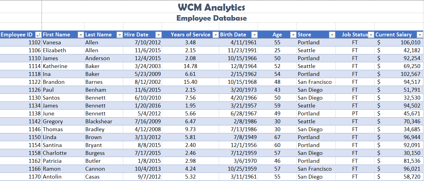
TABLE PROPERTIES & STRUCTURE
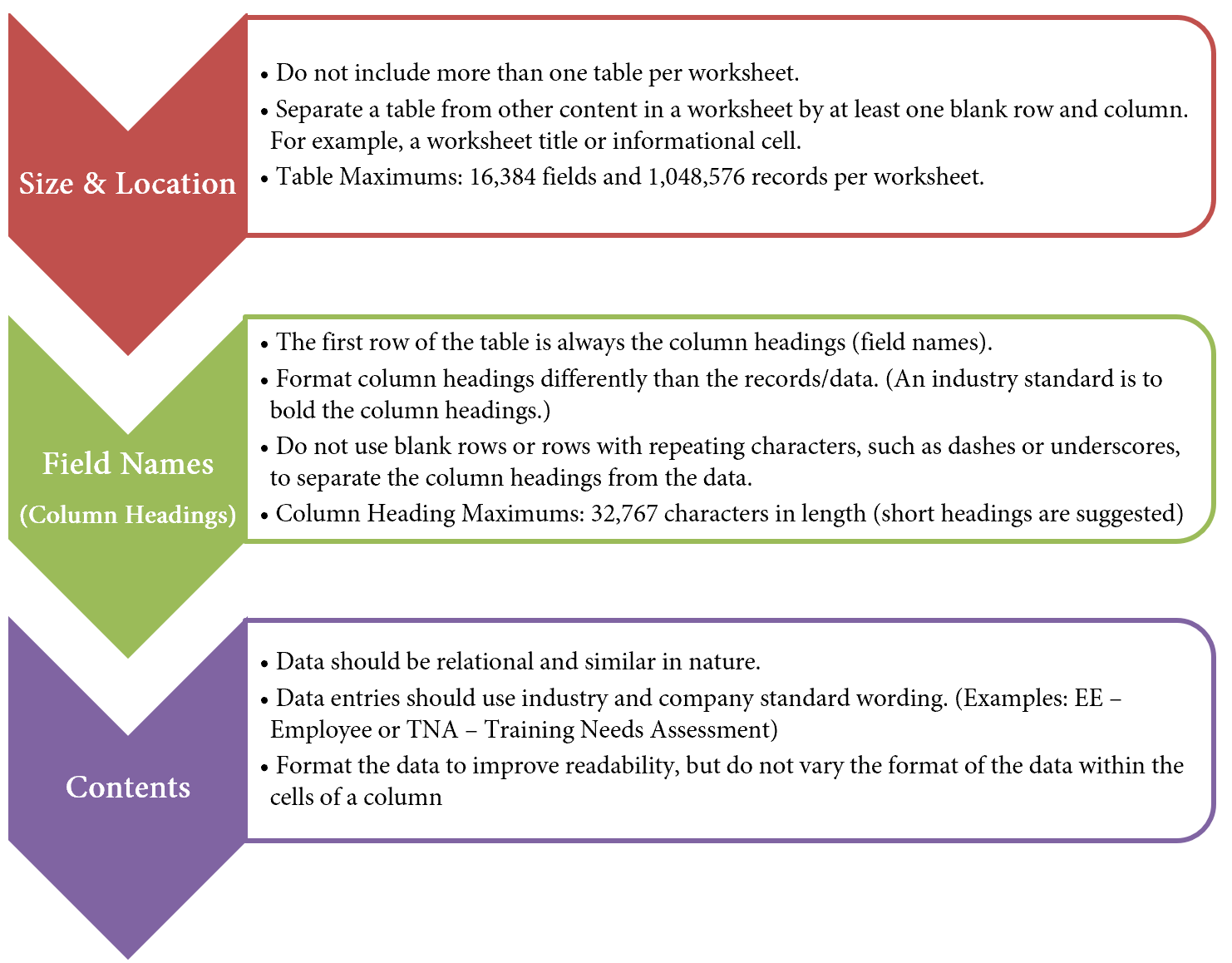
Turning a range of cells into an Excel table makes related data easier to analyze, visualize, and report. Structuring and planning table layouts are vital for data integrity. Below are guidelines to consider when designing and building a table from scratch:
OVERVIEW
Excel tables behave independently from the rest of the information on the worksheet. Excel treats the table area as a database locking the record entries together. There are several advantages of Excel treating the data independently. For example, using integrated filters and sort functions you can effortlessly drill down data based on questions and in return get results. Excel will also automatically expand the table to accommodate new data entries and allows for automatic formatting, such as recoloring of banded rows or columns.
You will also notice Excel treats formulas and calculations differently in a table, showing structured column names, along with automatically filling a calculated field to the entire table or offering quick and easy table totaling tools.
When graphing and charting table data you will also see Excel automatically adjusts of associated charts and ranges based on what the user is sorting or filtering at the time.
In industry, data is commonly stored in databases or multiple Excel files. Databases vary drastically, therefore in some cases, it is necessary to import data types into Excel. In our example, we will work with an Excel file that has imported data from a human resources database. The data downloaded from the database is stored in an Excel workbook, however, it’s in a Comma Separated Values (CSV) format. We will import the Excel file into our CH 5 Data file, turn the data into a table for further analysis.
IMPORT AND FORMAT DATA AS A TABLE
Download Data file: CH5 Data
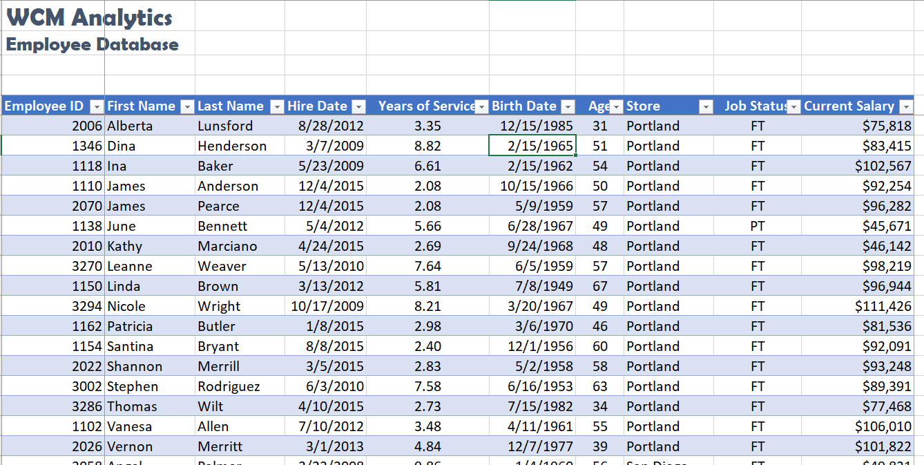
Keeping the above table guidelines in mind, import human resource data into Excel, as a table. Demonstrate tabling skills by examining employee relations, payroll, and benefits. Note you will need to save the CH 5 HR file on your computer as you will import this file into the CH 5 Data file in the below steps.
1. Open data file CH 5 Data and save the file as CH5 HR Report.
2. In the EmployeeData sheet, click on cell A5.
![]() Mac Users: Excel for Mac does not have the tool for “Getting Data” from an Excel Workbook. You will set up this data using alternate steps. Please skip steps 3-11. The alternate steps can be found below after Step 11.
Mac Users: Excel for Mac does not have the tool for “Getting Data” from an Excel Workbook. You will set up this data using alternate steps. Please skip steps 3-11. The alternate steps can be found below after Step 11.
3. From the Data tab, choose Get Data.
4. From the Get Data menu, choose From File, then From Workbook.
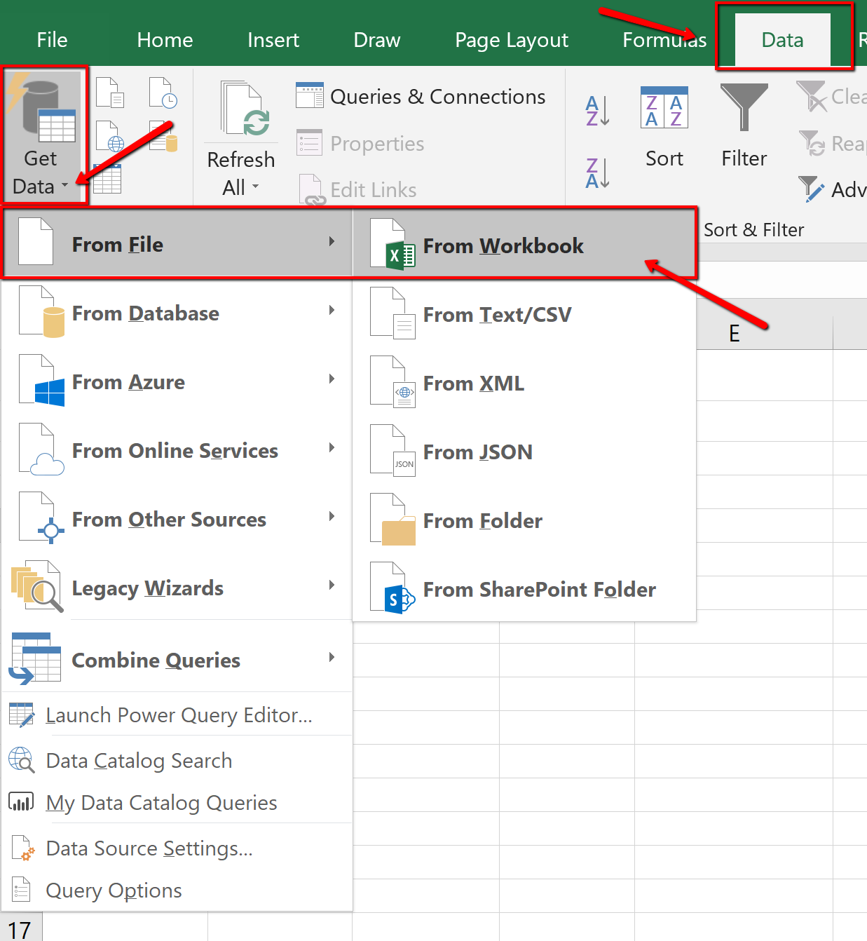
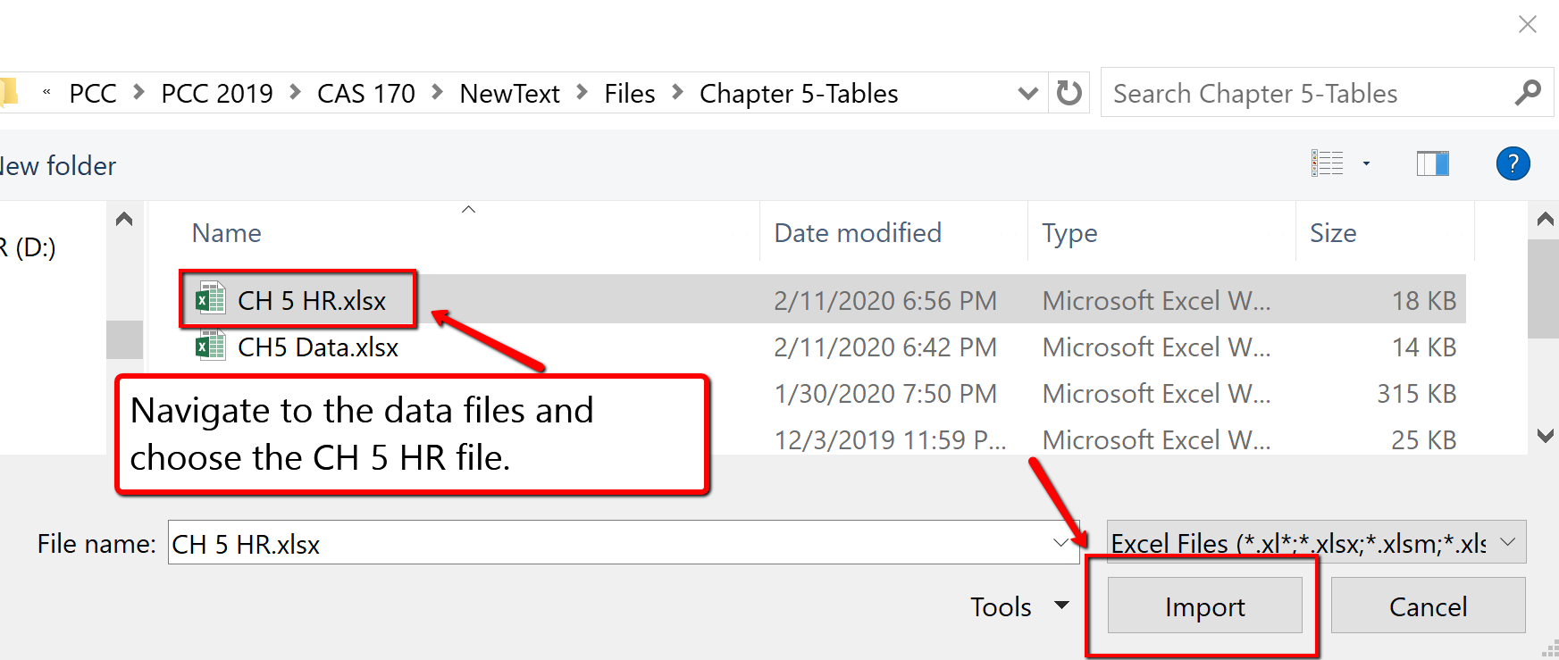
5. Navigate to the course data files. Find, and select the CH 5 HR file.
6. Click Import.
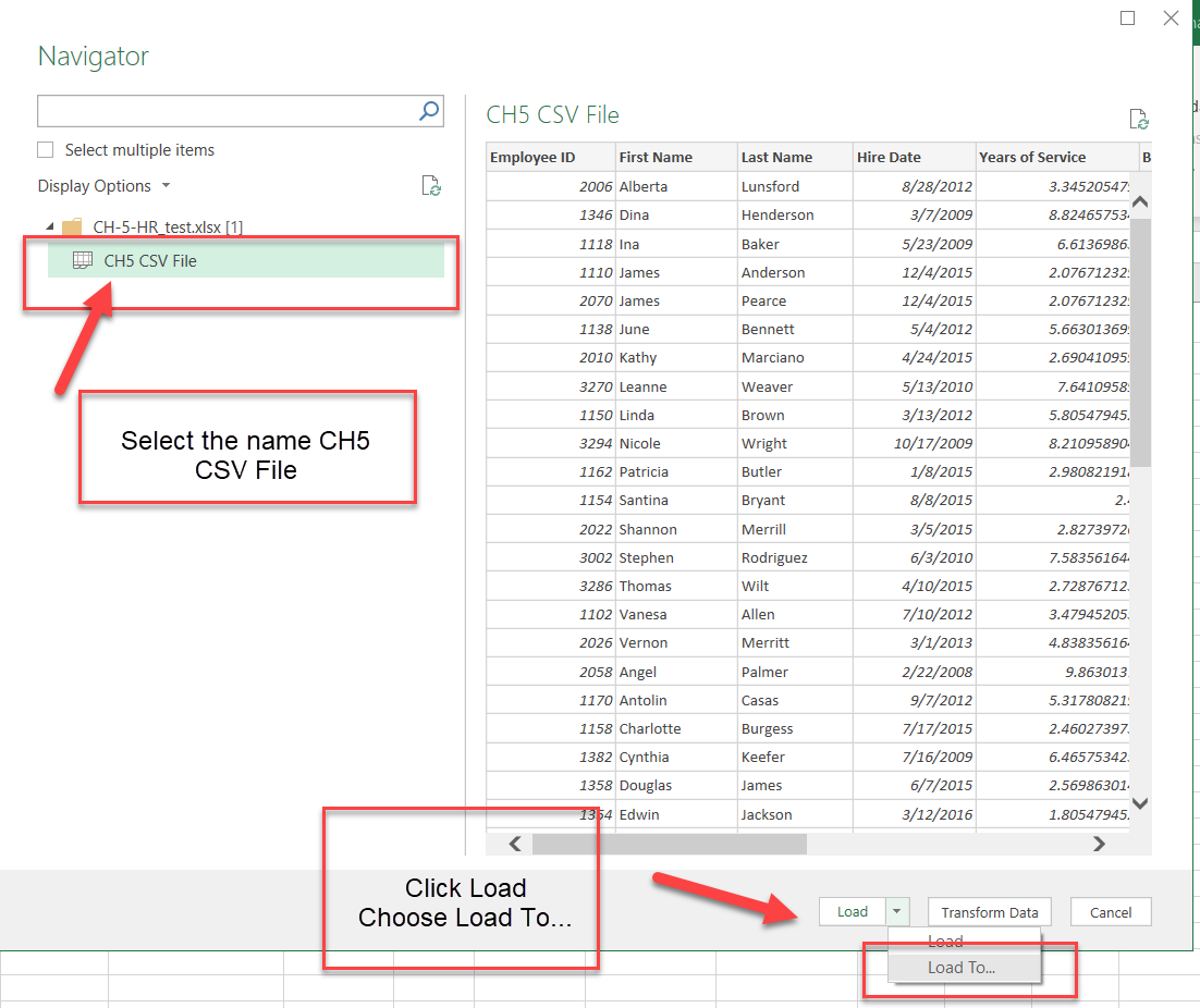
7. The Navigator dialogue box will open. Select the CH5 CSV File listed in the Display Options pane.
8. At the bottom of the Navigator dialogue box, select Load to expand the menu and choose Load To…
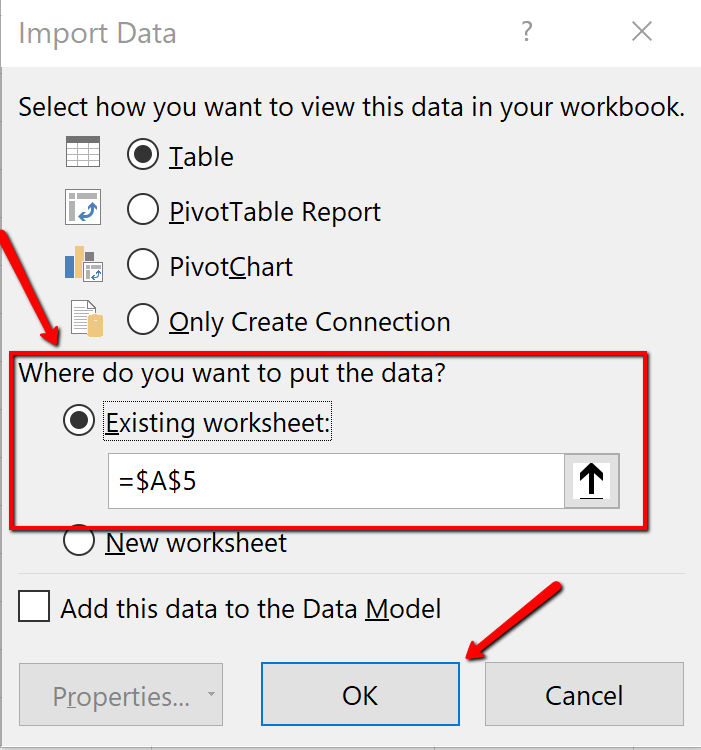
9. The Import dialogue box will open. In the “Where do you want to put the data?” section choose Existing worksheet:
10. In the above steps A5 was already selected when we started the import, so Excel will indicate we want the information to import and display starting at cell =$A$5. If you did not click cell A5, then select the cell now. Click OK.
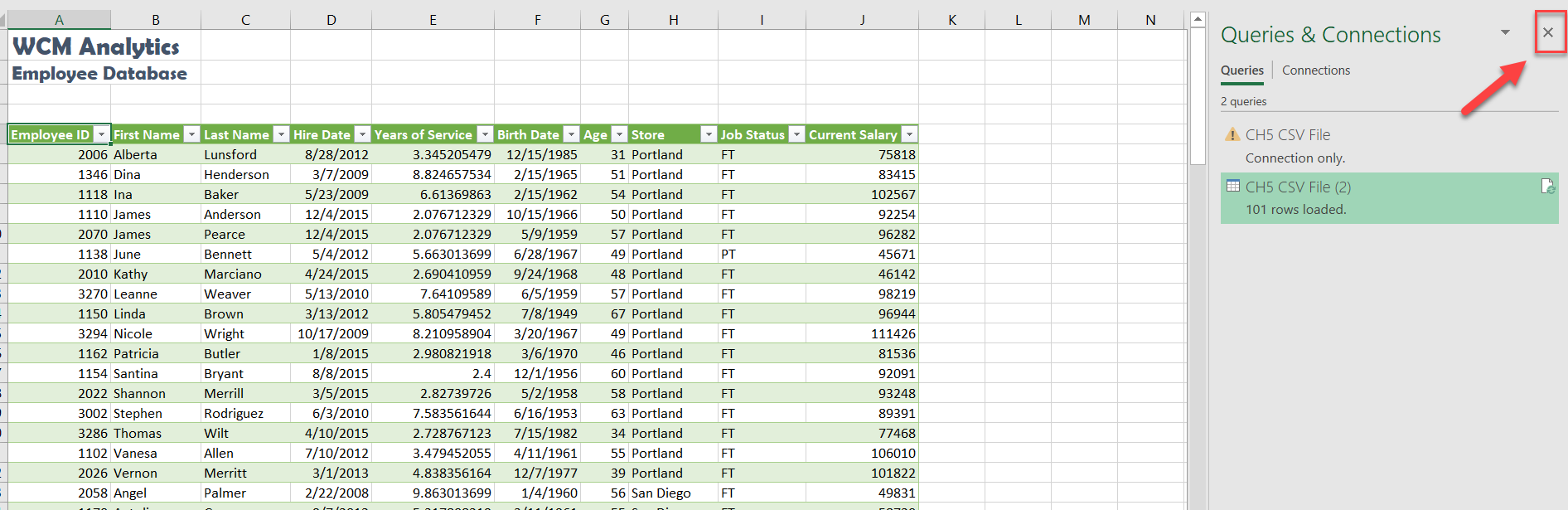
11. The data imports as a table. Close the Queries & Connections dialogue box.
![]() These are the alternate steps for Mac Users Only. If you are using Excel for Windows, please continue with the “Table Tools Design Tab” section below these alternate steps.
These are the alternate steps for Mac Users Only. If you are using Excel for Windows, please continue with the “Table Tools Design Tab” section below these alternate steps.
- Only complete the following steps if you are using a Mac. If you are using a PC, you have already inserted the table. You should already have the CH 5 HR Report open and you should have clicked into cell A5 in the EmploymentData sheet. If you did not do this, please do it now.
- Open the CH 5 HR workbook that you downloaded
- Use the keyboard shortcut of Ctrl key + letter A to select all of the data in the worksheet. That should be cells A1:J102
- Copy this data
- Switch back to the CH 5 Report workbook and make sure cell A5 is the active cell
- Paste the data into the Employment Data sheet at cell A5
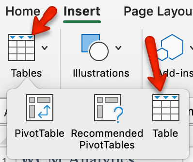
- Make sure Cell A5 is still the active cell and click the Insert tab from the Ribbon
- Click the Tables button from the Ribbon and then click the Tables icon
- The Create Table dialog box should appear with the cell range of A5:J106 as shown here in Figure 5.8. Click “OK” to accept this range for your table.
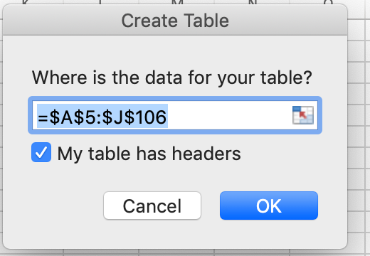
Figure 5.8 Excel for Mac Create Table Dialog Box - Congrats! You just converted the data to an Excel table. Continue following the steps in the section below.
TABLE TOOLS DESIGN TAB
Excel tables require specific tools. The Table Tools Design tab houses these specific tools used for formatting and editing tables. The Table Tools tab is considered a contextual tab; meaning the tabs appear when you are clicked in a table area. When you click out of a table, the Table Tools disappear.
Explore the table tools now. Notice the specific checkboxes to turn on table options, for example, you can choose to display banded rows or banded columns, or a total row etc. We will explore table tools in the following steps.
When importing data as a table, Excel automatically applied table formatting. Follow the below steps to format and edit the table.
1. Click the Table Tools/Design tab on the ribbon.
![]() Mac Users: you don’t have a Table Tools/Design tab. Just make sure the Table tab is selected.
Mac Users: you don’t have a Table Tools/Design tab. Just make sure the Table tab is selected.
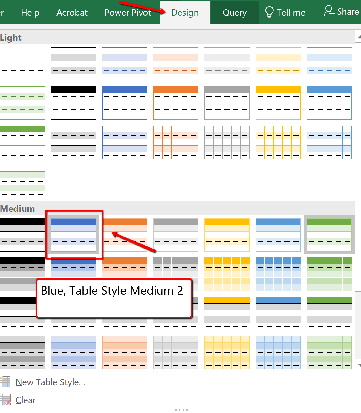
2. From the provided Table Styles, choose the Blue, Table Style Medium 2 option.
![]() Mac Users: the table you just created may already have the “Blue, Table Style Medium 2 option.
Mac Users: the table you just created may already have the “Blue, Table Style Medium 2 option.
Another option for inserting a table is using the Insert button. The Insert Table button, located on the Insert tab will turn a range of information into an unformatted table. We will use the insert table option later on in the chapter.
Skill Refresher
Format Data as a Table
- Click on the top-left cell in your data.
- Click the Format As Table menu from the Home tab on the Ribbon. Choose a style.
- Make sure “My table has headers” is checked. Click OK.
- Click on the top-left cell again.
- Adjust the widths of the columns so that you can see the complete headings with the filter arrows showing.
VIEWING table data
USING PANES
Data sets can bridge thousands of records with dozens of fields and extend beyond a workbook window. It can be difficult to compare fields and records in widely separated columns and rows. One way of dealing with this problem is by dividing the workbook window into viewing panes by using the Split view option. Excel can split the workbook window into four sections called panes with each pane offering a separate view into the worksheet. By scrolling through the contents of individual panes, you can compare cells from different sections of the worksheet side-by-side within the workbook window.
To split the workbook window into four panes, select any cell or range in the worksheet, and then on the View tab, in the Window group, click the Split button. Split bars divide the workbook window along the top and left border of the selected cell or range. To split the window into two vertical panes displayed side-by-side, select any cell in the first row of the worksheet and then click the Split button. To split the window into two stacked horizontal panes, select any cell in the first column and then click the Split button. To turn off the Spilt window option, simply click Split again on the View tab.
In our specific example the data set is manageable, however freezing the first column, and the top heading could be useful when scrolling through data.
FREEZE PANES
To keep an area of a worksheet visible while you scroll to another area of the worksheet use Freeze Panes. Follow the steps below to freeze, based on selection, the first column, and heading row.
1. If needed, adjust column widths so all heading names in row 5 are visible.
2. Click cell B6 in the table. (By selecting this specific cell, when we apply the freeze pane option, Excel will freeze the table where the first column ends and the heading row is viewable.)
3. Click the View tab.
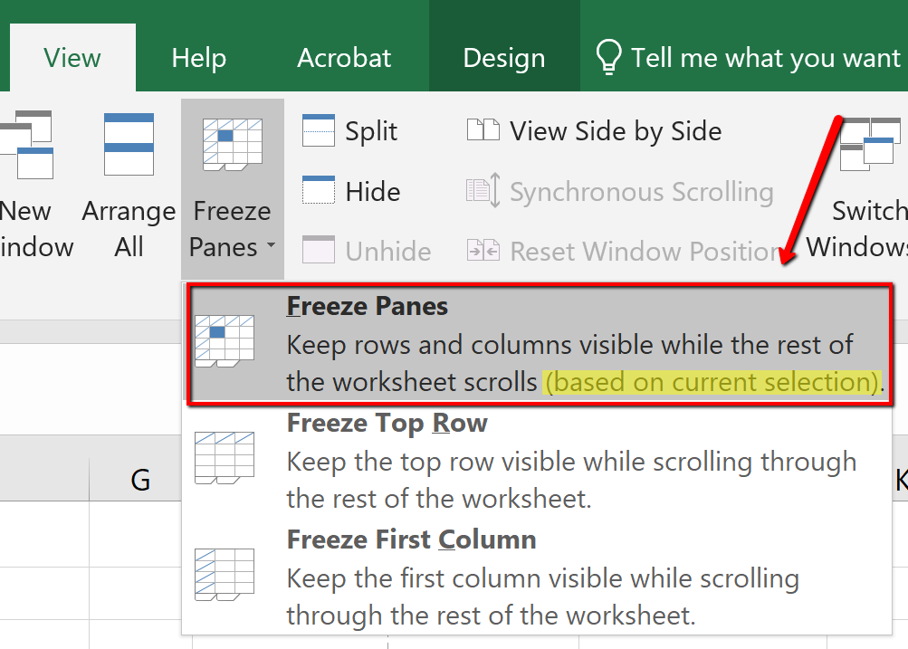
4. Select Freeze Panes, and for the listed options choose Freeze Panes (See Figure 5.10 below). The column and rows will remain visible based on the cell that was selected above.
![]() Mac Users should just click the Freeze Panes button
Mac Users should just click the Freeze Panes button 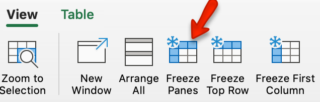 under the View tab.
Formatting table Data
After reviewing the table, two columns have data that need to be formatted accordingly. In large data sets, it is useful to know data selection short cuts. In this example, we are going to use keyboard short cuts to select a column of information in the table and apply number formatting.
Format data by following the below steps:
1. In the EmployeeData sheet, click cell E6.
2. On the keyboard press and hold the CTRL and SHIFT and DOWN keys.
3. With the “Years of Service” data selected, click the Home tab. In the Numbers category, format the data as a Number. The number should automatically decrease the decimal to two decimal places.
![]() Mac Users: click the “list arrow” next to “General,
Mac Users: click the “list arrow” next to “General, ![]() and then choose “Number” from the list.
and then choose “Number” from the list.
4. Click in cell J6. (Be sure you have clicked J6 so that you are in the first cell in the Current Salary column). Using the same selection process, select the Current Salary column, and format the data as Currency, zero decimal place.
5. Using the non-adjacent selection method, select column headings E, G, and I, and center the data.
NAMING A TABLE
Each time a table is created, Excel assigns a default name. The default naming convention is similar to the way new workbooks are named (Book1, Book2, etc.), however in this case Excel recognizes the area as a table and will assign the name table instead of book: Table1, Table2, Table3, and so on.
Why name a table range? Referring to the table by name rather than by range will make it easier to refer to a table in the future, for example, in a workbook that contains many tables. Seeing tables named Jan or Feb is more informational then seeing Table1 or Table 2. You can custom name each table and in the future connect named tables for reporting purposes.
There are two rules to consider when naming tables. One, Excel does not allow spaces in table names, and two, Excel also requires that table names begin with a letter or underscore.
Follow the next step to assign a custom name to the table.
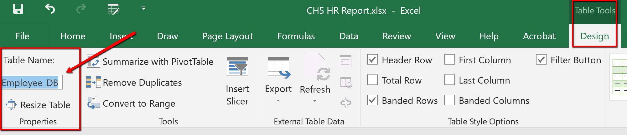
1. Click anywhere in the table and then display the Table Tools Design tab.
![]() Mac Users: there is no “Table Tools Design” tab in Excel for Mac. Simply click the Table tab and follow steps 2 and 3 below to give the table a new name.
Mac Users: there is no “Table Tools Design” tab in Excel for Mac. Simply click the Table tab and follow steps 2 and 3 below to give the table a new name.
2. Click the Table Name text box, in the Properties group.
3. Type Employee_DB and then press enter to name the table.
ENTERING & DELETING RECORDS
Tables require constant updating and may need calculations. When your table needs updating you can add/delete data, by adding/deleting rows, or columns. Excel adjusts the table automatically to the new content. The format applied to the banded rows updates to accommodate the new data set size.
When calculations are needed you can create a calculated column or use the built-in Total Row tool. Excel tables are a fantastic tool for entering formulas efficiently in a calculated column. Excel allows you to enter a single formula in one cell, and then that formula will automatically expand to the rest of the column by itself. There’s no need to use the Fill or Copy commands. This feature can be incredibly time-saving, especially if you have a lot of rows. And the same thing happens when you change a formula; the change will also expand to the rest of the calculated column. The Total Row tool, available on the Table Tools Design tab automatically adds a total row to the bottom of the table. To add a new row, uncheck the Total Row checkbox, add the row, and then recheck the Total Row checkbox. From the total row drop-down, you can select a function, like Average, Count, Count Numbers, Max, Min, Sum, StdDev, Var, and more.
Follow the steps below to update the employee table. You will insert new information just below the table. Data entered in rows or columns adjacent to the table becomes part of the table. Excel will format the new table data automatically.
1. Press and hold the Ctrl and End button to move to the last record in the table.
![]() Mac Users: there is no “End” key on most Mac keyboards. Press and hold the “Command” key and tap the right arrow key. Then press and hold the Command key, again, and tap the down arrow key. That should move to the last record in the table.
Mac Users: there is no “End” key on most Mac keyboards. Press and hold the “Command” key and tap the right arrow key. Then press and hold the Command key, again, and tap the down arrow key. That should move to the last record in the table.
2. Click tab to start a new record.
3. Type the new entries below. Click tab to move to the next column.
| 3297 | Alfred | Yelnats | 5/29/2015 | 2.59 | 2/19/1953 | 63 | Seattle | FT | $95,552 |
| 3299 | Jackson | Brown | 7/15/2013 | 4 | 3/16/1953 | 63 | Portland | FT | $98,655 |
As you enter the data, notice that Excel tries to complete your fields based on previous common entries.
REMOVE DUPLICATES
Duplicate entries may appear in tables. Why? Duplicates sometimes happen when data is entered incorrectly, by more than one person, or from more than one source. The following steps remove duplicate records in the table. In this particular table, Robert Griffin was entered twice by mistake. Delete the duplicate record by following the below steps:
1. Click anywhere in the table.
2. From the Table Tools Design tab click the Remove Duplicates button.
![]() Mac Users: Click the Table tab and click the Remove Duplicates button
Mac Users: Click the Table tab and click the Remove Duplicates button
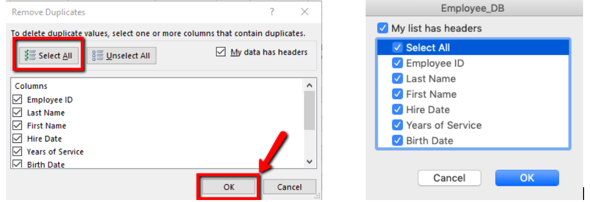
3. The Remove Duplicates dialog box will open.
4. If necessary, click the Select All button to deselect all columns.
5. Click OK to remove duplicate records from the table.
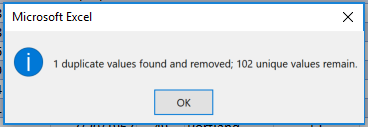
6. Excel notifies you that 1 duplicate record was removed.
CREATE NEW COLUMNS
In this next exercise, we will explore how to add two new columns in the table. Take note, Excel automatically adds the column to the table’s range and copies the format of the existing table heading to the new column heading. The first new column will use the VLOOKUP function to determine what cost of living adjustment (COLA) the employee qualifies for based on the region the employee lives in. The second column added will calculate the projected salary increase based on the COLA. When you use a formula in a table it is considered a calculated column.
A calculated column uses a single formula that adjusts for each row and automatically expands to include additional rows in that column. The formula is immediately extended to those rows. You only need to enter a formula to have it automatically filled down to create a calculated column—there’s no need to use the Fill or Copy commands.
As mentioned in the previous section, Excel assigns a name to the table, and to each column header in the table. When you add formulas to an Excel table, those names can appear automatically as you enter the formula and select the cell references in the table instead of manually entering them.
As a visual reference compare the differences to a formula entered in a cell, compared to in a table:
| Formula – Cell References | Formula – Table: Excel shows field names |
| =SUM(J6:K6) | =SUM([Current Salary]:[COLA]) |
Excel displaying table and or field names in a formula is called a structured reference. The names in structured references adjust whenever you add or remove data from the table headings. Structured references also appear when you create a formula outside of an Excel table that references table data. The references can make it easier to locate tables in a large workbook. To include structured references in your formula, use point mode method to click the cells you want to reference instead of typing their cell reference in the formula.
Complete the following steps to enter two new columns to determine each employee’s COLA and their projected salaries.
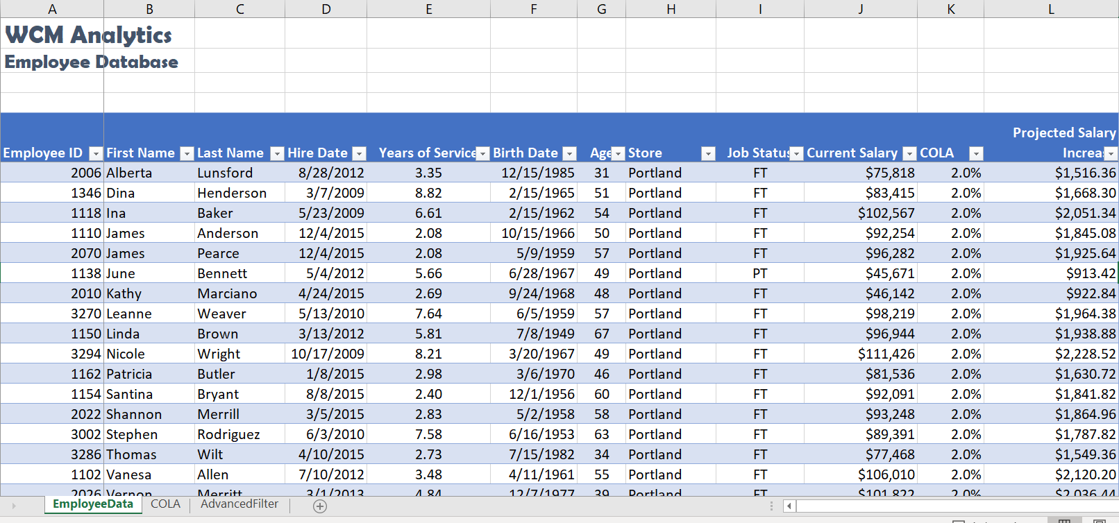
1. Click cell K5, and type COLA. Autofit the column width.
2. Click cell L5, and type Projected Salary Increase. Autofit the column width.
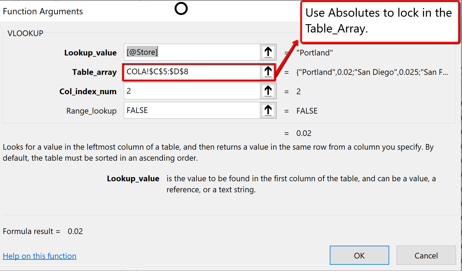
3. Click cell K6. From the Formulas tab, choose the VLOOKUP function (it is located within the “Lookup and Reference” tool) to look up each employee’s Store location. Matching their store location to the COLA table, located on the COLA sheet, bring over their percentage of increase listed in the second (2) column of the col_index. Note this is an EXACT match, so eliminate all FALSE possibilities in the Range_lookup area:
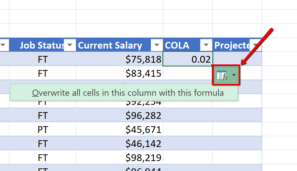
4. The Excel table will request you to overwrite all cells in the column with the formula. Click the icon, and choose the Overwrite command as shown below:
![]() Mac Users: Excel for Mac will automatically fill in the rest of the cells in the column. You do not have to click the icon. Close the Formula Builder pane.
Mac Users: Excel for Mac will automatically fill in the rest of the cells in the column. You do not have to click the icon. Close the Formula Builder pane.
5. Using point mode method click the table cells to calculate the employees Projected Salary Increase by multiplying the Current Salary by the COLA increase:
=[@[Current Salary]]*[@COLA]
6. The Excel table will again request you to overwrite all cells in the column with the formula. Click the icon, and choose the Overwrite command.
![]() Mac Users: You do not have to click the icon. Excel for Mac will auto-fill the rest of the cells in the column.
Mac Users: You do not have to click the icon. Excel for Mac will auto-fill the rest of the cells in the column.
7. Format the COLA and Projected Salary Increase columns by selecting K6:K107, and applying the percentage number format, and increase the decimal to one place. Autofit the column widths.
(Suggestion: Use the short cut selection method; click in K6, press and hold the CTRL and SHIFT and DOWN arrow keys to select the column data.)
8. Select L6:L107, and apply the Currency number format.
(Suggestion: Use the short cut selection method; click in L6, press and hold the CTRL and SHIFT and DOWN arrow keys to select the column data.)
9. Select L5. Wrap, and right-align the text, then decrease the column width, and increase the row height to show the contents of the heading row wrapped on two lines.
TOTAL ROW
A useful table tool for data analysis is the Total Row. You can quickly total data in an Excel table by enabling the Total Row option, and then use one of several built-in functions provided in a drop-down list, per column. The Total row, which is added to the end of the table after the last data record can calculate summary statistics, including the average, sum, minimum, and maximum of select fields within the table. The Total row is formatted with values displayed in bold, the double border line option is separating the data records from the Total row.
Apply a Total Row, and follow the below steps to sum three columns of data:
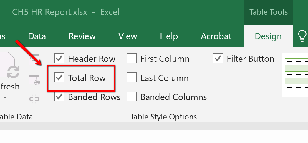
- Click anywhere in the table and choose the Table Tools Design tab, and click on the Total Row option.
![]() Mac Users: just click the Table tab and click on the Total Row option
Mac Users: just click the Table tab and click on the Total Row option
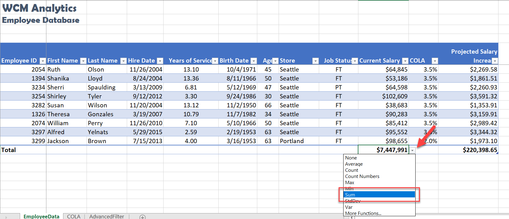
2. Excel redirects you to the bottom of the table to view the total row, where a SUM defaulted in the Projected Salary Increase column. Click cell J108, select choose the Total Row menu arrow. Choose SUM to total the Current Salary column.
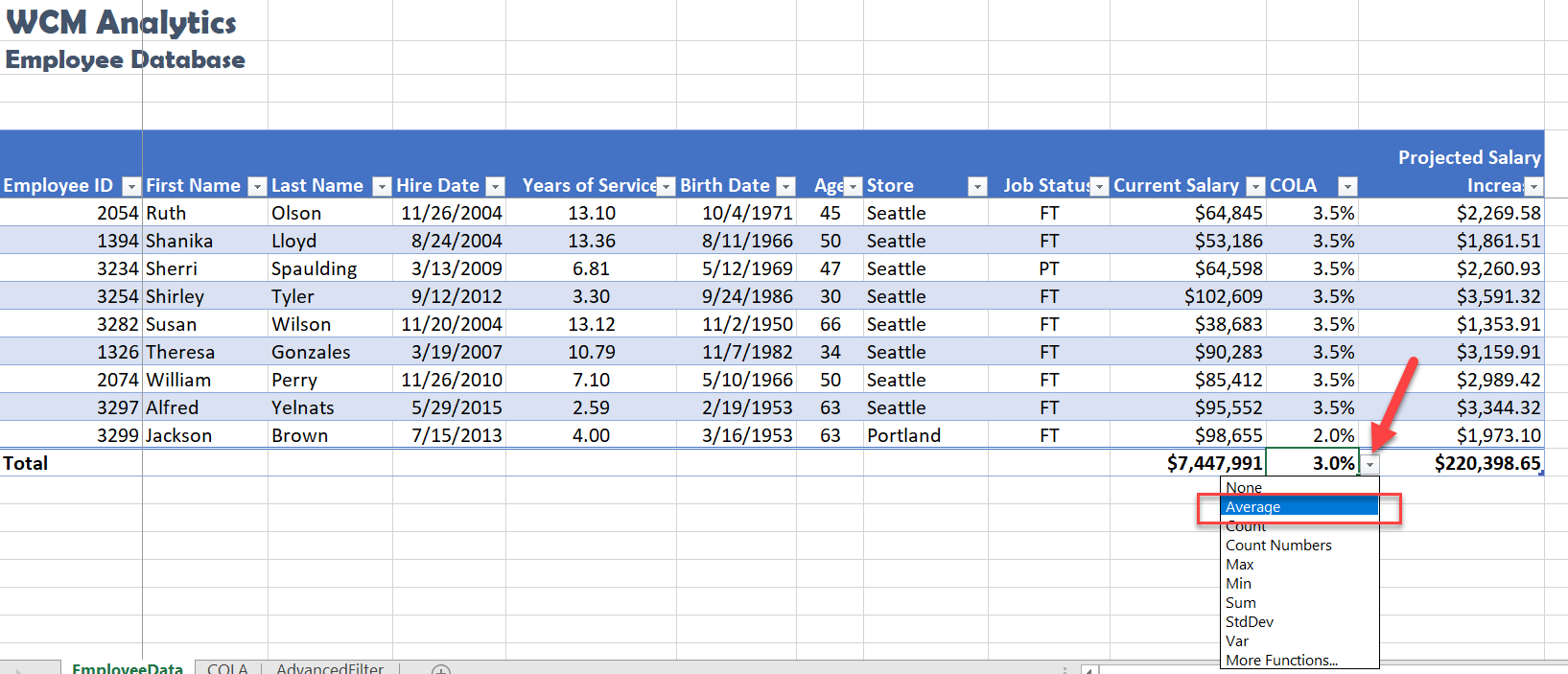
3. Click cell K108, from the total row menu select Average. The average COLA increase will display.
CENTER ACROSS SELECTION
Follow the below steps to center the title in cell A1:L2 using the Center Across Selection tool located in the Format Cells dialog box. In prior chapters, we used the ‘Merge & Center’ button to center text across a range. The Merge & Center tool centers the title but removes access to individual cells. This restriction can present a problem when trying to autofit column widths in a table. The Center Across Selection format centers text across multiple cells but does not merge the selected cell range into one cell making it a better formatting choice when working with tables.
1. Select cell A1:L2, and right-click to access the short cut menu.
![]() Mac Users: hold down CTRL key and click the selected cells to access the short cut menu
Mac Users: hold down CTRL key and click the selected cells to access the short cut menu
2. Choose Format Cells.
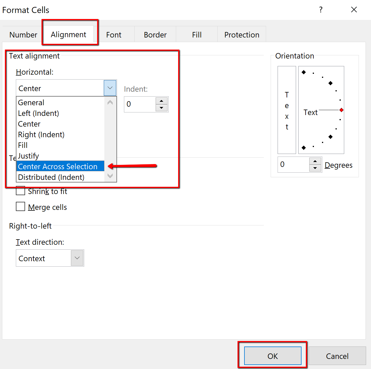
3. In the Format Cells dialogue box, choose the Alignment tab.
4. From the Horizontal alignment menu, choose Center Across Selection. Click OK to return to the table.
Attribution
“5.1 Table Basics” by Hallie Puncochar, Portland Community College is licensed under CC BY 4.0
