
Learning Objectives
- Calculate the price elasticity of demand
- Calculate the price elasticity of supply
Both the demand and supply curve show the relationship between price and the number of units demanded or supplied. Price elasticity is the ratio between the percentage change in the quantity demanded (Qd) or supplied (Qs) and the corresponding percent change in price. The price elasticity of demand is the percentage change in the quantity demanded of a good or service divided by the percentage change in the price. The price elasticity of supply is the percentage change in quantity supplied divided by the percentage change in price.
Elasticities can be usefully divided into three broad categories: elastic, inelastic, and unitary. An elastic demand or elastic supply is one in which the elasticity is greater than one, indicating a high responsiveness to changes in price. Elasticities that are less than one indicate low responsiveness to price changes and correspond to inelastic demand or inelastic supply. Unitary elasticities indicate proportional responsiveness of either demand or supply, as summarized in Table 1.
| If: | Then: | And It Is Called: |
|---|---|---|
| [latex]\%\;change\;in\;quantity > \%\;change\;in\;price[/latex] | [latex]\frac{\%\;change\;in\;quantity}{\%\;change\;in\;price)} > 1[/latex] | Elastic |
| [latex]\%\;change\;in\;quantity = \%\;change\;in\;price[/latex] | [latex]\frac{\%\;change\;in\;quantity}{\%\;change\;in\;price)} = 1[/latex] | Unitary |
| [latex]\%\;change\;in\;quantity \%\;change\;in\;price[/latex] | [latex]\frac{\%\;change\;in\;quantity}{\%\;change\;in\;price)} 1[/latex] | Inelastic |
| Table 1. Elastic, Inelastic, and Unitary: Three Cases of Elasticity | ||
Before we get into the nitty gritty of elasticity, enjoy this article on elasticity and ticket prices at the Super Bowl.

To calculate elasticity, instead of using simple percentage changes in quantity and price, economists use the average percent change in both quantity and price. This is called the Midpoint Method for Elasticity, and is represented in the following equations:
The advantage of the is Midpoint Method is that one obtains the same elasticity between two price points whether there is a price increase or decrease. This is because the formula uses the same base for both cases.
Calculating Price Elasticity of Demand
Let’s calculate the elasticity between points A and B and between points G and H shown in Figure 1.
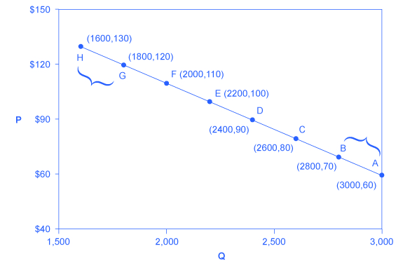
First, apply the formula to calculate the elasticity as price decreases from $70 at point B to $60 at point A:
Therefore, the elasticity of demand between these two points is [latex]\frac { 6.9\% }{ -15.4\% }[/latex] which is 0.45, an amount smaller than one, showing that the demand is inelastic in this interval. Price elasticities of demand are always negative since price and quantity demanded always move in opposite directions (on the demand curve). By convention, we always talk about elasticities as positive numbers. So mathematically, we take the absolute value of the result. We will ignore this detail from now on, while remembering to interpret elasticities as positive numbers.
This means that, along the demand curve between point B and A, if the price changes by 1%, the quantity demanded will change by 0.45%. A change in the price will result in a smaller percentage change in the quantity demanded. For example, a 10% increase in the price will result in only a 4.5% decrease in quantity demanded. A 10% decrease in the price will result in only a 4.5% increase in the quantity demanded. Price elasticities of demand are negative numbers indicating that the demand curve is downward sloping, but are read as absolute values. The following Work It Out feature will walk you through calculating the price elasticity of demand.
Finding the Price Elasticity of Demand
Calculate the price elasticity of demand using the data in Figure 1 for an increase in price from G to H. Has the elasticity increased or decreased?
Step 1. We know that:
Step 2. From the Midpoint Formula we know that:
Step 3. So we can use the values provided in the figure in each equation:
Step 4. Then, those values can be used to determine the price elasticity of demand:
Therefore, the elasticity of demand from G to H 1.47. The magnitude of the elasticity has increased (in absolute value) as we moved up along the demand curve from points A to B. Recall that the elasticity between these two points was 0.45. Demand was inelastic between points A and B and elastic between points G and H. This shows us that price elasticity of demand changes at different points along a straight-line demand curve.
Calculating the Price Elasticity of Supply
Assume that an apartment rents for $650 per month and at that price 10,000 units are rented as shown in Figure 2. When the price increases to $700 per month, 13,000 units are supplied into the market. By what percentage does apartment supply increase? What is the price sensitivity?
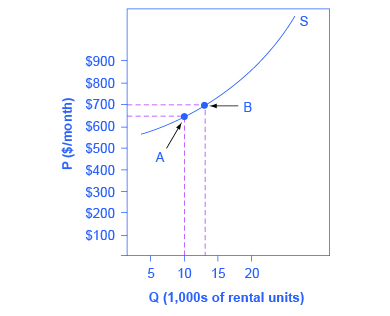
Using the Midpoint Method,
Again, as with the elasticity of demand, the elasticity of supply is not followed by any units. Elasticity is a ratio of one percentage change to another percentage change—nothing more—and is read as an absolute value. In this case, a 1% rise in price causes an increase in quantity supplied of 3.5%. The greater than one elasticity of supply means that the percentage change in quantity supplied will be greater than a one percent price change. If you're starting to wonder if the concept of slope fits into this calculation, read the following Clear It Up box.
Is the elasticity the slope?
It is a common mistake to confuse the slope of either the supply or demand curve with its elasticity. The slope is the rate of change in units along the curve, or the rise/run (change in y over the change in x). For example, in Figure 1, each point shown on the demand curve, price drops by $10 and the number of units demanded increases by 200. So the slope is –10/200 along the entire demand curve and does not change. The price elasticity, however, changes along the curve. Elasticity between points A and B was 0.45 and increased to 1.47 between points G and H. Elasticity is the percentage change, which is a different calculation from the slope and has a different meaning.
When we are at the upper end of a demand curve, where price is high and the quantity demanded is low, a small change in the quantity demanded, even in, say, one unit, is pretty big in percentage terms. A change in price of, say, a dollar, is going to be much less important in percentage terms than it would have been at the bottom of the demand curve. Likewise, at the bottom of the demand curve, that one unit change when the quantity demanded is high will be small as a percentage.
So, at one end of the demand curve, where we have a large percentage change in quantity demanded over a small percentage change in price, the elasticity value would be high, or demand would be relatively elastic. Even with the same change in the price and the same change in the quantity demanded, at the other end of the demand curve the quantity is much higher, and the price is much lower, so the percentage change in quantity demanded is smaller and the percentage change in price is much higher. That means at the bottom of the curve we'd have a small numerator over a large denominator, so the elasticity measure would be much lower, or inelastic.
As we move along the demand curve, the values for quantity and price go up or down, depending on which way we are moving, so the percentages for, say, a $1 difference in price or a one unit difference in quantity, will change as well, which means the ratios of those percentages will change.
Key Concepts and Summary
Price elasticity measures the responsiveness of the quantity demanded or supplied of a good to a change in its price. It is computed as the percentage change in quantity demanded (or supplied) divided by the percentage change in price. Elasticity can be described as elastic (or very responsive), unit elastic, or inelastic (not very responsive). Elastic demand or supply curves indicate that quantity demanded or supplied respond to price changes in a greater than proportional manner. An inelastic demand or supply curve is one where a given percentage change in price will cause a smaller percentage change in quantity demanded or supplied. A unitary elasticity means that a given percentage change in price leads to an equal percentage change in quantity demanded or supplied.
Self-Check Questions
- From the data shown in Table 2 about demand for smart phones, calculate the price elasticity of demand from: point B to point C, point D to point E, and point G to point H. Classify the elasticity at each point as elastic, inelastic, or unit elastic.
Points P Q A 60 3,000 B 70 2,800 C 80 2,600 D 90 2,400 E 100 2,200 F 110 2,000 G 120 1,800 H 130 1,600 Table 2. - From the data shown in Table 3 about supply of alarm clocks, calculate the price elasticity of supply from: point J to point K, point L to point M, and point N to point P. Classify the elasticity at each point as elastic, inelastic, or unit elastic.
Point Price Quantity Supplied J $8 50 K $9 70 L $10 80 M $11 88 N $12 95 P $13 100 Table 3.
Review Questions
- What is the formula for calculating elasticity?
- What is the price elasticity of demand? Can you explain it in your own words?
- What is the price elasticity of supply? Can you explain it in your own words?
Critical Thinking Questions
- Transatlantic air travel in business class has an estimated elasticity of demand of 0.40 less than transatlantic air travel in economy class, with an estimated price elasticity of 0.62. Why do you think this is the case?
- What is the relationship between price elasticity and position on the demand curve? For example, as you move up the demand curve to higher prices and lower quantities, what happens to the measured elasticity? How would you explain that?
Problems
- The equation for a demand curve is P = 48 – 3Q. What is the elasticity in moving from a quantity of 5 to a quantity of 6?
- The equation for a demand curve is P = 2/Q. What is the elasticity of demand as price falls from 5 to 4? What is the elasticity of demand as the price falls from 9 to 8? Would you expect these answers to be the same?
- The equation for a supply curve is 4P = Q. What is the elasticity of supply as price rises from 3 to 4? What is the elasticity of supply as the price rises from 7 to 8? Would you expect these answers to be the same?
- The equation for a supply curve is P = 3Q – 8. What is the elasticity in moving from a price of 4 to a price of 7?
Glossary
- elastic demand
- when the elasticity of demand is greater than one, indicating a high responsiveness of quantity demanded or supplied to changes in price
- elastic supply
- when the elasticity of either supply is greater than one, indicating a high responsiveness of quantity demanded or supplied to changes in price
- elasticity
- an economics concept that measures responsiveness of one variable to changes in another variable
- inelastic demand
- when the elasticity of demand is less than one, indicating that a 1 percent increase in price paid by the consumer leads to less than a 1 percent change in purchases (and vice versa); this indicates a low responsiveness by consumers to price changes
- inelastic supply
- when the elasticity of supply is less than one, indicating that a 1 percent increase in price paid to the firm will result in a less than 1 percent increase in production by the firm; this indicates a low responsiveness of the firm to price increases (and vice versa if prices drop)
- price elasticity
- the relationship between the percent change in price resulting in a corresponding percentage change in the quantity demanded or supplied
- price elasticity of demand
- percentage change in the quantity demanded of a good or service divided the percentage change in price
- price elasticity of supply
- percentage change in the quantity supplied divided by the percentage change in price
- unitary elasticity
- when the calculated elasticity is equal to one indicating that a change in the price of the good or service results in a proportional change in the quantity demanded or supplied
Solutions
Answers to Self-Check Questions
- From point B to point C, price rises from $70 to $80, and Qd decreases from 2,800 to 2,600. So:
[latex]\begin{array}{r @{{}={}} l}\%\;change\;in\;quantity & \frac { { 2,600 }-{ 2,800 } }{ ({ 2,600 }+{ 2,800 })/2 } \times 100 \\[1em] & \frac { -200 }{ 2,700 } \times 100 \\[1em] & -7.41 \\[1em] \%\;change\;in\;price & \frac { { 80 }-{ 70 } }{ ({ 80 }+{ 70 })/2 } \times 100 \\[1em] & \frac { 10 }{ 75 } \times 100 \\[1em] & 13.33 \\[1em] Elasticity\;of\;Demand & \frac { -7.41\% }{ 13.33\% } \\[1em] & 0.56 \end{array}[/latex]
The demand curve is inelastic in this area; that is, its elasticity value is less than one.
Answer from Point D to point E:
[latex]\begin{array}{r @{{}={}} l}\%\;change\;in\;quantity & \frac { { 2,200 }-{ 2,400 } }{ ({ 2,200 }+{ 2,400 })/2 } \times 100 \\[1em] & \frac { -200 }{ 2,300 } \times 100 \\[1em] & -8.7 \\[1em] \%\;change\;in\;price & \frac { { 100 }-{ 90 } }{ ({ 100 }+{ 90 })/2 } \times 100 \\[1em] & \frac { 10 }{ 95 } \times 100 \\[1em] & 10.53 \\[1em] Elasticity\;of\;Demand & \frac { -8.7\% }{ 10.53\% } \\[1em] & 0.83 \end{array}[/latex]The demand curve is inelastic in this area; that is, its elasticity value is less than one.
Answer from Point G to point H:
[latex]\&s=4 \begin{array}{r @{{}={}} l}\%\;change\;in\;quantity & \frac { { 1,600 }-{ 1,800 } }{ ({ 1,600 }+{ 1,800 })/2 } \times 100 \\[1em] & \frac { -200 }{ 1,700 } \times 100 \\[1em] & -11.76 \\[1em] \%\;change\;in\;price & \frac { { 130 }-{ 120 } }{ ({ 130 }+{ 120 })/2 } \times 100 \\[1em] & \frac { 10 }{ 125 } \times 100 \\[1em] & 7.81 \\[1em] Elasticity\;of\;Demand & \frac { -11.76\% }{ 7.81\% } \\[1em] & -1.51 \end{array}[/latex]The demand curve is elastic in this interval.
- From point J to point K, price rises from $8 to $9, and quantity rises from 50 to 70. So:
[latex]\begin{array}{r @{{}={}} l}\%\;change\;in\;quantity & \frac { { 70 }-{ 50 } }{ ({ 70 }+{ 50 })/2 } \times 100 \\[1em] & \frac { 20 }{ 60 } \times 100 \\[1em] & 33.33 \\[1em] \%\;change\;in\;price & \frac { { \$9 }-{ \$8 } }{ ({ \$9 }+{ \$8 })/2 } \times 100 \\[1em] & \frac { 1 }{ 8.5 } \times 100 \\[1em] & 11.76 \\[1em] Elasticity\;of\;Supply & \frac { 33.33\% }{ 11.76\% } \\[1em] & 2.83 \end{array}[/latex]
The supply curve is elastic in this area; that is, its elasticity value is greater than one.
From point L to point M, the price rises from $10 to $11, while the Qs rises from 80 to 88:
[latex]\begin{array}{r @{{}={}} l}\%\;change\;in\;quantity & \frac { { 88 }-{ 80 } }{ ({ 88 }+{ 80 })/2 } \times 100 \\[1em] & \frac { 8 }{ 84 } \times 100 \\[1em] & 9.52 \\[1em] \%\;change\;in\;price & \frac { { \$11 }-{ \$10 } }{ ({ \$11 }+{ \$10 })/2 } \times 100 \\[1em] & \frac { 1 }{ 10.5 } \times 100 \\[1em] & 9.52 \\[1em] Elasticity\;of\;Demand & \frac { 9.52\% }{ 9.52\% } \\[1em] & 1.0 \end{array}[/latex]The supply curve has unitary elasticity in this area.
From point N to point P, the price rises from $12 to $13, and Qs rises from 95 to 100:
[latex]\&s=4 \begin{array}{r @{{}={}} l}\%\;change\;in\;quantity & \frac { { 100 }-{ 95 } }{ ({ 100 }+{ 95 })/2 } \times 100 \\[1em] & \frac { 5 }{ 97.5 } \times 100 \\[1em] & 5.13 \\[1em] \%\;change\;in\;price & \frac { { \$13 }-{ \$12 } }{ ({ \$13 }+{ \$12 })/2 } \times 100 \\[1em] & \frac { 1 }{ 12.5 } \times 100 \\[1em] & 8.0 \\[1em] Elasticity\;of\;Supply & \frac { 5.13\% }{ 8.0\% } \\[1em] & 0.64 \end{array}[/latex]The supply curve is inelastic in this region of the supply curve.
