
5.5 Scored Assessment
Tables for a Retail Company
Download Data File: SC5 Data
Retail companies with today’s online, as well as, in-store sales have a lot of data to keep track of! Keeping track of sales, costs, and profits on a daily basis is essential to making the most of a business. This exercise illustrates how to use the skills presented in this chapter to generate the data needed on a daily basis by a retail company. See Figure 5.31 above.
- Open the data file SC5 Data and save the file to your computer as SC5 Dynamite Customer Sales.
- Click on the Sales sheet. In I4 , enter a VLOOKUP function that will find the Product Price for the Product in E4 in the table in the Product Table sheet and return it to I4. In your VLOOKUP function, fill in the required parameters using Figure 5.32 below. Copy the VLOOKUP function down column I.
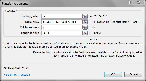
Figure 5.32 VLOOKUP window - In J4 , enter a VLOOKUP function that will find the Product Cost for the Product in E4 in the table in the Product Table sheet and return it to J4. This VLOOKUP function will be the same as the VLOOKUP function in I4 – EXCEPT THE COL_INDEX_NUM will be 3 instead of 4. Copy the function down column J.
- In K4, calculate Profit (Product Price – Product Cost). Copy this formula down column K.
- Format columns I, J, and K as currency with two decimal places.
- Click in cell A3. Insert a table with headers for the range A3:K52. BE CAREFUL HERE: Excel will try to insert a table starting with A2. You want to make sure your range starts with A3 here.
- Make a copy of the Sales sheet and rename it Online Sales by Date. Place this sheet to the right of the Sales sheet. Filter out Retail in Sales Type, so that only Online Sales are displayed. Sort the filtered data by Date Sold (oldest to newest).
- Make a copy of the Sales sheet and rename it June Sales by Country. Place this new sheet to the right of the Online Sales by Date sheet. Filter this sheet to only show June dates by using the Date Filter Between. Sort this sheet alphabetically (A to Z) by Country and then alphabetically by Name.
- Make another copy of the Sales sheet and rename it Sales by Product. Place this new sheet to the right of the June Sales by Country sheet. Hide the Region column.
- Insert a slicer in the Sales by Product sheet for Product Sold. Move the top left corner of the slicer to the top left-hand corner of cell M1. Resize the height of the entire slicer to 2.09”.
- Select both DETA100 and DETA200 in the slicer. Sort the filtered sheet by Product Sold. Add a Total Row that includes the overall average for the Product Price, Product Cost, and Profit columns. Change the heading in A53 to Average.
- Make a copy of the Sales sheet and rename it Subtotals by Date. Place this new sheet to the right of the Sales by Product sheet. Subtotal the sheet by Date (Oldest to Newest), summing the Profit column. Click the 2 Outline button to show just the subtotals by date and the grand total.
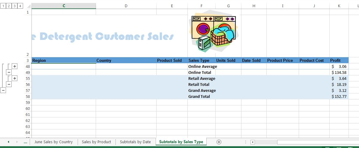
- Make one final copy of the Sales sheet and rename it Subtotals by Type. Place this new sheet to the right of the Subtotals by Date sheet. Subtotal the sheet by Sales Type, summing the Profit column.
- Add a 2nd subtotal to the Subtotals by Type sheet that subtotals by Type and averages the Profit column. (Hint: uncheck Replace Current Subtotals in the Subtotal dialog box.) Notice that 4 Outline buttons appear with the 2nd subtotal. Figure out which Outline button to click to display both subtotals for Online and Retail and two Grand Totals.
- For each worksheet, add a footer with the worksheet name in the center.
- Preview each worksheet in Print Preview and make any necessary changes for professional printing. (Hint: Orientation, page scaling, and print titles might need to be used)
- Double-check that your sheets are in the following order from left to right: Sales, Online Sales by Date, June Sales by Country, Sales by Product, Subtotals by Date, Subtotals by Sales Type, and Product Table.
- Save the SC5 Dynamite Customer Sales workbook.
- Submit the SC5 Dynamite Customer Sales workbook as directed by your instructor.
Attribution
“5.5 Scored Assessment” by Diane Shingledecker, Portland Community College is licensed under CC BY 4.0
