
4.2 Population Growth and Regulation
Population ecologists make use of a variety of methods to model population dynamics. An accurate model should be able to describe the changes occurring in a population and predict future changes.
Population Growth
The two simplest models of population growth use deterministic equations (equations that do not account for random events) to describe the rate of change in the size of a population over time. The first of these models, exponential growth, describes populations that increase in numbers without any limits to their growth. The second model, logistic growth, introduces limits to reproductive growth that become more intense as the population size increases. Neither model adequately describes natural populations, but they provide points of comparison.
Exponential Growth
Charles Darwin, in developing his theory of natural selection, was influenced by the English clergyman Thomas Malthus. Malthus published his book in 1798 stating that populations with abundant natural resources grow very rapidly. However, they limit further growth by depleting their resources. The early pattern of accelerating population size is called exponential growth (Figure 1).
The best example of exponential growth in organisms is seen in bacteria. Bacteria are prokaryotes that reproduce quickly, about an hour for many species. If 1000 bacteria are placed in a large flask with an abundant supply of nutrients (so the nutrients will not become quickly depleted), the number of bacteria will have doubled from 1000 to 2000 after just an hour. In another hour, each of the 2000 bacteria will divide, producing 4000 bacteria. After the third hour, there should be 8000 bacteria in the flask. The important concept of exponential growth is that the growth rate—the number of organisms added in each reproductive generation—is itself increasing; that is, the population size is increasing at a greater and greater rate. After 24 of these cycles, the population would have increased from 1000 to more than 16 billion bacteria. When the population size, N, is plotted over time, a J-shaped growth curve is produced (Figure 1).
The bacteria-in-a-flask example is not truly representative of the real world where resources are usually limited. However, when a species is introduced into a new habitat that it finds suitable, it may show exponential growth for a while. In the case of the bacteria in the flask, some bacteria will die during the experiment and thus not reproduce; therefore, the growth rate is lowered from a maximal rate in which there is no mortality.
Logistic Growth
Extended exponential growth is possible only when infinite natural resources are available; this is not the case in the real world. Charles Darwin recognized this fact in his description of the “struggle for existence,” which states that individuals will compete, with members of their own or other species, for limited resources. The successful ones are more likely to survive and pass on the traits that made them successful to the next generation at a greater rate (natural selection). To model the reality of limited resources, population ecologists developed the logistic growth model.
Carrying Capacity and the Logistic Model
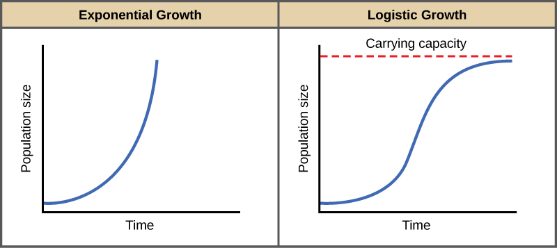
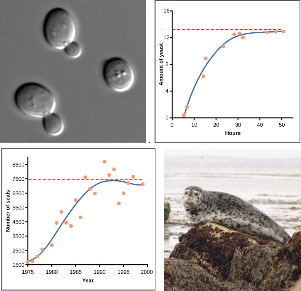
In the real world, with its limited resources, exponential growth cannot continue indefinitely. Exponential growth may occur in environments where there are few individuals and plentiful resources, but when the number of individuals gets large enough, resources will be depleted and the growth rate will slow down. Eventually, the growth rate will plateau or level off (Figure 1). This population size, which is determined by the maximum population size that a particular environment can sustain, is called the carrying capacity, symbolized as K. In real populations, a growing population often overshoots its carrying capacity and the death rate increases beyond the birth rate causing the population size to decline back to the carrying capacity or below it. Most populations usually fluctuate around the carrying capacity in an undulating fashion rather than existing right at it.
A graph of logistic growth yields the S-shaped curve (Figure 1). It is a more realistic model of population growth than exponential growth. There are three different sections to an S-shaped curve. Initially, growth is exponential because there are few individuals and ample resources available. Then, as resources begin to become limited, the growth rate decreases. Finally, the growth rate levels off at the carrying capacity of the environment, with little change in population number over time.
Examples of Logistic Growth
Population Dynamics and Regulation
The logistic model of population growth, while valid in many natural populations and a useful model, is a simplification of real-world population dynamics. Implicit in the model is that the carrying capacity of the environment does not change, which is not the case. The carrying capacity varies annually. For example, some summers are hot and dry whereas others are cold and wet; in many areas, the carrying capacity during the winter is much lower than it is during the summer. Also, natural events such as earthquakes, volcanoes, and fires can alter an environment and hence its carrying capacity. Additionally, populations do not usually exist in isolation. They share the environment with other species, competing with them for the same resources (interspecific competition). These factors are also important to understanding how a specific population will grow.
Why Did the Woolly Mammoth Go Extinct?
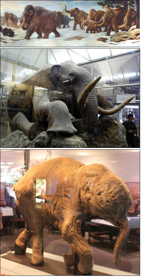
Most populations of woolly mammoths went extinct about 10,000 years ago, soon after paleontologists believe humans began to colonize North America and northern Eurasia (Figure 3). A mammoth population survived on Wrangel Island, in the East Siberian Sea, and was isolated from human contact until as recently as 1700 BC. We know a lot about these animals from carcasses found frozen in the ice of Siberia and other northern regions.
It is commonly thought that climate change and human hunting led to their extinction. A 2008 study estimated that climate change reduced the mammoth’s range from 3,000,000 square miles 42,000 years ago to 310,000 square miles 6,000 years ago.2 Through archaeological evidence of kill sites, it is also well documented that humans hunted these animals. A 2012 study concluded that no single factor was exclusively responsible for the extinction of these magnificent creatures.3 In addition to climate change and reduction of habitat, scientists demonstrated another important factor in the mammoth’s extinction was the migration of human hunters across the Bering Strait to North America during the last ice age 20,000 years ago.
The maintenance of stable populations was and is very complex, with many interacting factors determining the outcome. It is important to remember that humans are also part of nature. Once we contributed to a species’ decline using primitive hunting technology only.
Demographic-Based Population Models
Population ecologists have hypothesized that suites of characteristics may evolve in species that lead to particular adaptations to their environments. These adaptations impact the kind of population growth their species experience. Life history characteristics such as birth rates, age at first reproduction, the numbers of offspring, and even death rates evolve just like anatomy or behavior, leading to adaptations that affect population growth. Population ecologists have described a continuum of life-history “strategies” with K-selected species on one end and r-selected species on the other. K-selected species are adapted to stable, predictable environments. Populations of K-selected species tend to exist close to their carrying capacity. These species tend to have larger, but fewer, offspring and contribute large amounts of resources to each offspring. Elephants would be an example of a K-selected species. r-selected species are adapted to unstable and unpredictable environments. They have large numbers of small offspring. Animals that are r-selected do not provide a lot of resources or parental care to offspring, and the offspring are relatively self-sufficient at birth. Examples of r-selected species are marine invertebrates such as jellyfish and plants such as the dandelion. The two extreme strategies are at two ends of a continuum on which real species life histories will exist. In addition, life history strategies do not need to evolve as suites, but can evolve independently of each other, so each species may have some characteristics that trend toward one extreme or the other.
Attribution
Population Dynamics and Regulation by OpenStax is licensed under CC BY 4.0. Modified from the original by Matthew R. Fisher.
