
Equilibrium with Unemployment
Learning Objectives
By the end of this section, you will be able to:
- Evaluate the Keynesian view of recessions and the effect of wage and price adjustments
- Explain the determination of equilibrium using the Keynesian Cross Model
- Analyze the impact of the expenditure multiplier
- Explain the heterodox view of unemployment equilibrium
Now that we have a clear understanding of how aggregate demand is understood in the Keynesian model, we can look to what this model tells us about capitalist economies. In this section, you will learn about how a free market economy will react to situations of excess aggregate supply or aggregate demand. Before returning to the Keynesian cross model, however, it is worth looking into why this approach is fundamentally different from orthodox economics.
Rejecting Equilibration through Wage and Price Adjustments
In the opening pages of the General Theory, Keynes questioned the orthodox model of free market economies, specifically as it concerns the role of wage adjustments in reducing unemployment. Recall that, in the standard orthodox model of labor markets, (involuntary) unemployment exists when the supply of labor exceeds the demand for labor; and this excess supply exists when wages (the price of labor) are above equilibrium. It follows, then, that a reduction of wages should solve the unemployment problem of a recession. The issue with this argument–and this should be intuitive if you think about it–is that, in a period in which workers are being laid off because business’ sales are down, if the people who still had jobs saw their paychecks shrink, the obvious result would be lower sales and more layoffs. But this is precisely the opposite of the prediction from the orthodox model.
The same could be said for price declines when firms see sales (demand) dropping below their production levels (supply). The standard (orthodox) market model suggests that lower prices would encourage more purchases and hence higher sales. Unfortunately, most businesses in most industries know that these sorts of desperate price cuts can drive everyone into bankruptcy. The reason is simple: lower prices means lower revenues, which means lower margins and therefore less money to cover current expenses and recoup (and earn a profit on) past investments.
The takeaway from all of this is that the orthodox model of the macroeconomy is deeply flawed. It’s not only the case that, in a recession, wage and price declines would not improve the situation, they’d actually make things worse. This argument deals a heavy blow to orthodox economics which believes that price (including wage) adjustments make up the essential coordinating mechanism–the invisible hand–of free market economies. In fact, as Keynes and many heterodox economists before and after him have argued, price changes simply do not play the basic equilibrating role–that is, the function of balancing all the different parts of the economy–that orthodox economists believe they do. Below, we’ll look at a simple alternative mechanism for macroeconomic equilibrium: not price, but quantity adjustments in the face of excess aggregate supply or aggregate demand.
Equilibrium in the Keynesian Cross Model
With the aggregate expenditure line in place, the next step in understanding our Keynesian cross diagram is to relate it to the two other elements of the model. Thus, the first subsection below interprets the intersection of the aggregate expenditure function and the 45-degree line, while the next subsection relates this point of intersection to the potential GDP line.
Where Equilibrium Occurs
The point where the aggregate expenditure line that is constructed from C + I + G + X – M crosses the 45-degree line will be the equilibrium for the economy. It is the only point on the aggregate expenditure line where the total amount being spent on aggregate demand equals the total level of production. In Figure 7 of the previous section this point of equilibrium (E0) happens at 6,000, which can also be read off Table 3.
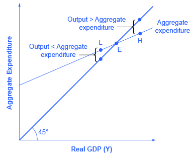
The meaning of “equilibrium” remains the same; that is, equilibrium is a point of balance where no incentive exists to shift away from that outcome. To understand why the point of intersection between the aggregate expenditure function and the 45-degree line is a macroeconomic equilibrium, consider what would happen if an economy found itself to the right of the equilibrium point E, say point H in Figure 1, below, where output is higher than the equilibrium. At point H, the level of aggregate expenditure is below the 45-degree line, so that the level of aggregate expenditure in the economy is less than the level of output. As a result, at point H, output is piling up unsold—not a sustainable state of affairs. Recall that, in this model, the adjustment mechanism is output, not price. Let’s assume for simplicity that prices don’t change at all. What do you think businesses will do when they find that they’re not selling what they had produced?
Say you owned and managed a restaurant and, on a Saturday evening that you had expected to be busy, you ended up seeing only a few people coming in to dine. Certainly you’re not going to be cooking as many meals as you had expected–since, after all, there simply aren’t as may people ordering meals as you had expected. Most likely you’re also going to respond by sending unneeded cooks and waitstaff home. In the Keynesian Model, we’re assuming this is generally what happens when, in the aggregate, there is less demand than supply: firms respond by reducing output and laying off workers. This will, in turn, reduce spending, moving us backwards along the aggregate expenditure curve in the figure above.
So, as a result of too little spending relative to output, output is cut. But this cuts income, too, which means spending will decline. The trick here is that some of that income lost from the layoffs would have been saved, which means that the lost spending will be less than the lost output. You can see this graphically in the figure above by watching the gap between the two curves shrink as we move from point H back toward point E.
Conversely, consider the situation where the level of output is at point L—where real output is lower than the equilibrium. In that case, the level of aggregate demand in the economy is above the 45-degree line, indicating that the level of aggregate expenditure in the economy is greater than the level of output. When the level of aggregate demand is so high that the store shelves have been emptied, the economy is also in an unsustainable situation. Firms will respond by increasing their level of production, hiring more people (for instance, calling a cook who had the day off in to work). This, in turn, will increase income, which will increase spending–though, because some of that income will be saved, spending won’t rise as fast as output.
Thus, the equilibrium must be the point where the amount produced and the amount spent are in balance, at the intersection of the aggregate expenditure function and the 45-degree line. This is the macroeconomic equivalent to the restaurant that scheduled just the right number of cooks, waitstaff, and so on for the number of customers who actually came in to eat.
The Expenditure Multiplier
A key concept in Keynesian economics is the expenditure multiplier. The expenditure multiplier is the idea that not only does spending affect the equilibrium level of GDP, but that spending is powerful. More precisely, it means that a change in spending causes a more than proportionate change in GDP.
[latex]\frac{\text{$\Delta$ Y}}{\text{$\Delta$ Spending}}>1[/latex]
The reason for the expenditure multiplier is that one person’s spending becomes another person’s income, which leads to additional spending and additional income so that the cumulative impact on GDP is larger than the initial increase in spending. While the multiplier is important for understanding the effectiveness of fiscal policy, it occurs whenever any autonomous increase in spending occurs. Additionally, the multiplier operates in a negative as well as a positive direction. Thus, when investment spending collapsed during the Great Depression, it caused a much larger decrease in real GDP. The size of the multiplier is critical and was a key element in discussions of the effectiveness of the Obama administration’s fiscal stimulus package, officially titled the American Recovery and Reinvestment Act of 2009.
Finally, with a few simplifying examples, we can reduce the algebra you’ve studied above to one simple equation for the equilibrium level of output (and income and expenditures). Assume that there is no government (spending nor taxing) and no foreign sector (imports nor exports). In this case, equilibrium output can be expressed simply in terms of the marginal propensity to consume, autonomous consumption, and investment:
Note that, since (1-mpc) is the same as the marginal propensity to save, we could also write this equation as:
[latex]Y=\frac{1}{mps}\times(C_a + I)[/latex]
Note that the first term in the right-hand side of these equations ([latex]\frac{1}{1-mpc}[/latex] or [latex]\frac{1}{mps}[/latex]) is the same as our expenditure multiplier. That is, this part of the equation tells us by how much output will increase (or decrease) if one of the other components, autonomous consumption or investment were to increase (or decrease).
Unemployment Equilibrium
At this point, you should be able to able to construct the Keynesian cross diagram, including the 45 degree line and the aggregate expenditure curve. You should also be able to identify, both graphically and algebraically, the equilibrium level of output and income. But what about full employment? Recall that, in the orthodox model of aggregate supply/aggregate demand, full employment was ensured through flexible prices in the factor markets (including labor). If the economy were ever operating at less than full employment, adjustments in the prices of these inputs would move it back to full employment–at least, in the long run. Where do Keynes and the heterodox economies working within similar frameworks stand on the free market and full employment?
The short answer is that Keynes and most heterodox economists simply reject the idea that capitalist economies will normally be at–or moving toward–full employment. Simply put, there’s no reason to think that the level of aggregate expenditure in the economy will be just right to ensure that everyone who wants to work gets a job (and all other productive resources are being used as well. And this goes back to how employment decisions are made: if there are sales, then production and employment will happen; if there aren’t sales, there’s no reason to produce, no work to do.
Ultimately, then, we have to ask, do businesses and consumers make there spending decisions based on the national unemployment rate? Generally, no. You and I don’t consult the Bureau of Labor Statistics before we decide whether to go out to eat, and neither do businesses before they decide to expand or replace worn out equipment. (Technically, you can imagine a consumer or a business seeing high unemployment and getting worried about spending. But this isn’t likely to make lead them to fix the problem by spending more. In fact, it’s likely to make them spend less, which of course would only make a bad unemployment situation worse.)
So this is a crucial point of distinction between orthodox economists, using the aggregate supply/aggregate demand model, and heterodox economists using the Keynesian model: while orthodox economists believe, at least in the long run, the economy will tend toward a full employment equilibrium, heterodox economists only believe that it will tend toward some equilibrium. Technically, heterodox economists argue, that equilibrium could be at full employment; but there’s no reason to expect this to be the normal case. In fact, it would probably be quite abnormal.
Summary
The great insights of Keynes’ General Theory as we’ve covered thus far can be summarized by two main ideas: (1) demand drives supply, and (2) when the economy is in disequilibrium, its primarily output that adjusts, not prices. In this and the previous section, you’ve learned that from these insights we can build a relatively simple model of aggregate expenditures and the process of attaining macroeconomic equilibrium. Importantly, from the heterodox perspective that Keynes was a part of, there is no reason to expect that this equilibrium would be consistent with the full employment of the economy’s labor and other resources.
Glossary
- expenditure multiplier
- Keynesian concept that asserts that a change in autonomous spending causes a more than proportionate change in real GDP
a model in the heterodox tradition of Keynes that shows aggregate expenditure as a function of income and equilibrium at the point where spending and output are equal
Keynesian concept that asserts that a change in autonomous spending causes a more than proportionate change in real GDP
