
Using Fiscal Policy to Fight Recession, Unemployment, and Inflation
Learning Objectives
By the end of this section, you will be able to:
- Explain how expansionary fiscal policy can shift aggregate demand and influence the economy
- Explain how contractionary fiscal policy can shift aggregate demand and influence the economy
Fiscal policy is the use of government spending and tax policy to influence the path of the economy over time. At its most basic, fiscal policy operates through increasing aggregate demand (expansionary fiscal policy) or decreasing aggregate demand (contractionary fiscal policy). In this section you will see how expansionary and contractionary fiscal policy affect the economy by looking at both the aggregate demand/aggregate supply model as well as the Keynesian cross model.
Fiscal Policy and Growth in the Aggregate Demand/Aggregate Supply Model
Graphically, we see that fiscal policy, whether through changes in spending or taxes, shifts the aggregate demand outward in the case of expansionary fiscal policy and inward in the case of contractionary fiscal policy. We know from the chapter on economic growth that over time the quantity and quality of our resources grow as the population and thus the labor force get larger, as businesses invest in new capital, and as technology improves. The result of this is regular shifts to the right of the aggregate supply curves, as Figure 1 illustrates.
The original equilibrium occurs at E0, the intersection of aggregate demand curve AD0 and aggregate supply curve SRAS0, at an output level of 200 and a price level of 90. One year later, aggregate supply has shifted to the right to SRAS1 in the process of long-term economic growth, and aggregate demand has also shifted to the right to AD1, keeping the economy operating at the new level of potential GDP. The new equilibrium (E1) is an output level of 206 and a price level of 92. One more year later, aggregate supply has again shifted to the right, now to SRAS2, and aggregate demand shifts right as well to AD2. Now the equilibrium is E2, with an output level of 212 and a price level of 94. In short, the figure shows an economy that is growing steadily year to year, producing at its potential GDP each year, with only small inflationary increases in the price level.

Aggregate demand and aggregate supply do not always move neatly together. Think about what causes shifts in aggregate demand over time. As aggregate supply increases, incomes tend to go up. This tends to increase consumer and investment spending, shifting the aggregate demand curve to the right, but in any given period it may not shift the same amount as aggregate supply. What happens to government spending and taxes? Government spends to pay for the ordinary business of government- items such as national defense, social security, and healthcare, as Figure 1 shows. Tax revenues then reduce private incomes and hence spending. The result may be an increase in aggregate demand more than or less than the increase in aggregate supply.
Aggregate demand may fail to increase along with aggregate supply, or aggregate demand may even shift left, for a number of possible reasons: households become hesitant about consuming; firms decide against investing as much; or perhaps the demand from other countries for exports diminishes.
For example, investment by private firms in physical capital in the U.S. economy boomed during the late 1990s, rising from 14.1% of GDP in 1993 to 17.2% in 2000, before falling back to 15.2% by 2002. Conversely, if shifts in aggregate demand run ahead of increases in aggregate supply, inflationary increases in the price level will result. Business cycles of recession and recovery are the consequence of shifts in aggregate supply and aggregate demand. As these occur, the government may choose to use fiscal policy to address the difference.
Monetary Policy and Bank Regulation shows us that a central bank can use its powers over the banking system to engage in countercyclical—or “against the business cycle”—actions. If recession threatens, the central bank uses an expansionary monetary policy to increase the money supply, increase the quantity of loans, reduce interest rates, and shift aggregate demand to the right. If inflation threatens, the central bank uses contractionary monetary policy to reduce the money supply, reduce the quantity of loans, raise interest rates, and shift aggregate demand to the left. Fiscal policy is another macroeconomic policy tool for adjusting aggregate demand by using either government spending or taxation policy.
Expansionary fiscal policy increases the level of aggregate demand, through either increases in government spending or reductions in tax rates. Expansionary policy can do this by (1) increasing consumption by raising disposable income through cuts in personal income taxes or payroll taxes; (2) increasing investment spending by raising after-tax profits through cuts in business taxes; and (3) increasing government purchases through increased federal government spending on final goods and services and raising federal grants to state and local governments to increase their expenditures on final goods and services. Contractionary fiscal policy does the reverse: it decreases the level of aggregate demand by decreasing consumption, decreasing investment, and decreasing government spending, either through cuts in government spending or increases in taxes. The aggregate demand/aggregate supply model as well as the Keynesian cross model can be useful in judging whether expansionary or contractionary fiscal policy is appropriate.
The Aggregate Demand/Aggregate Supply Model
Consider first the situation in Figure 2 which is similar to the U.S. economy during the 2008-2009 recession. The intersection of aggregate demand (AD0) and aggregate supply (SRAS0) is occurring below the level of potential GDP as the LRAS curve indicates. At the equilibrium (E0), a recession occurs and unemployment rises. In this case, expansionary fiscal policy using tax cuts or increases in government spending can shift aggregate demand to AD1, closer to the full-employment level of output. In addition, the price level would rise back to the level P1 associated with potential GDP.

Fiscal policy can also contribute to pushing aggregate demand beyond potential GDP in a way that leads to inflation. As Figure 3 shows, a very large budget deficit pushes up aggregate demand, so that the intersection of aggregate demand (AD0) and aggregate supply (SRAS0) occurs at equilibrium E0, which is an output level above potential GDP. Economists sometimes call this an “overheating economy” where demand is so high that there is upward pressure on wages and prices, causing inflation. In this situation, contractionary fiscal policy involving federal spending cuts or tax increases can help to reduce the upward pressure on the price level by shifting aggregate demand to the left, to AD1, and causing the new equilibrium E1 to be at potential GDP, where aggregate demand intersects the LRAS curve.

Again, the AD–AS model does not dictate how the government should carry out this contractionary fiscal policy. Some may prefer spending cuts; others may prefer tax increases; still others may say that it depends on the specific situation. The model only argues that, in this situation, the government needs to reduce aggregate demand.
The Keynesian Cross Model
In many of their basic elements, both the Ad-AS model and the Keynesian cross model are similar when it comes to analyzing fiscal policy. In both, expansionary fiscal policy increases aggregate demand (or aggregate expenditure) and contractionary fiscal policy decreases it. However, where the AD-AS model includes changes in the price level, the Keynesian model holds prices constant. But, where the AD-AS model only looks at a given change in aggregate demand, the Keynesian model includes the multiplier effect whereby an initial change in government spending (or taxes) has an even greater impact on the level of output and income in the economy as a whole.
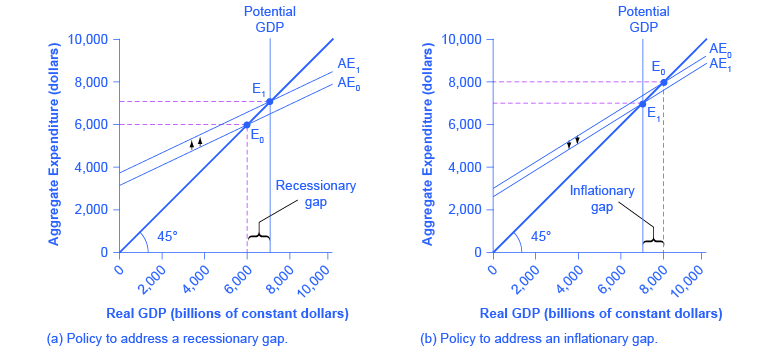
As you’ve seen in a previous chapter, we can think of the function of fiscal policy as closing the recessionary gap or the inflationary gap, as the case may be. Expansionary fiscal policy would be appropriate for closing a recessionary gap, raising the aggregate expenditure function from AE0 to AE1 in the first panel below. Likewise, contractionary fiscal policy would be appropriate for closing an inflationary gap, lowing the aggregate expenditure function from AE0 to AE1 in the second panel below.
We can demonstrate these ideas algebraically as well. Recall that the equilibrium output and income in an economy with no public or foreign sectors can be expressed as:
[latex]Y=\frac{1}{mps}\times(C_a + I)[/latex]
Where the mps is the marginal propensity to save, Ca is autonomous consumption, and I is investment.
Now, suppose that we calculate equilibrium output and income (Y), given that the mps = 0.5, autonomous consumption = 2,000, and investment = 1,000, as follows:
[latex]Y=\frac{1}{0.5}\times(2000 + 1000) = 2\times3000 = 6000[/latex]
Now suppose that we believed that potential GDP is at 7,000, in which case there is a recessionary gap of 1,000. You’ll recall that because of the multiplier effect, the economy doesn’t need $1,000 of new spending to close the gap. Instead it only needs 1,000 divided by the multiplier (2). We can show this through the expansionary fiscal policy of a government spending (G) increase of $500:
[latex]Y=\frac{1}{mps}\times(C_a + I + G)[/latex]
Then
[latex]Y=\frac{1}{0.5}\times(2000 + 1000 + 500) = 2\times3500 = 7000[/latex]
Naturally, a tax cut would also be capable of closing the gap. Without complicating the algebra too much further, we can ask: by how much would taxes need to be cut to get the same impact as our $500 increase in government spending? The complication here is that some of the increase in disposable income that households would enjoy from a tax cut would be saved.
In the example above, the mps is 0.5 so, 50 cents of every dollar of a tax cut would not be spent, and hence would not increase output at all. What this tells us is that we would need a tax cut that, when multiplied by the marginal propensity to consume (telling us how much of that income would actually be spent), gives us the $500 spending increase we need. Hence,
[latex]\text{Tax Cut}=\frac{\text{Increased Spending Needed}}{mpc}[/latex]
In this case, that comes out to:
[latex]\frac{500}{0.5}=1000[/latex]
So, because only half of it will be spent (the other half saved) a $1,000 tax cut will result in an initial increase of $500 of spending, which will then multiply through to increase output and income by $1,000, just like the $500 increase in government spending.
To Increase Spending or to Cut Taxes?
Should the government use tax cuts or spending increases, or a mix of the two, to carry out expansionary fiscal policy? During the 2008-2009 Great Recession (which started, actually, in late 2007), the U.S. economy suffered a 3.1% cumulative loss of GDP. That may not sound like much, but it’s more than one year’s average growth rate of GDP. Over that time frame, the unemployment rate doubled from 5% to 10%. The consensus view is that this was possibly the worst economic downturn in U.S. history since the 1930’s Great Depression. The choice between whether to use tax or spending tools often has a political tinge. As a general statement, conservatives and Republicans prefer to see expansionary fiscal policy carried out by tax cuts, while liberals and Democrats prefer that the government implement expansionary fiscal policy through spending increases. In a bipartisan effort to address the extreme situation, the Obama administration and Congress passed an $830 billion expansionary policy in early 2009 involving both tax cuts and increases in government spending. At the same time, however, the federal stimulus was partially offset when state and local governments, whose budgets were hard hit by the recession, began cutting their spending.
The conflict over which policy tool to use can be frustrating to those who want to categorize economics as “liberal” or “conservative,” or who want to use economic models to argue against their political opponents. However, advocates of smaller government, who seek to reduce taxes and government spending can use the models we’ve been working with, as well as advocates of bigger government, who seek to raise taxes and government spending. Economic studies of specific taxing and spending programs can help inform decisions about whether the government should change taxes or spending, and in what ways. Ultimately, decisions about whether to use tax or spending mechanisms to implement macroeconomic policy is a political decision well as an economic one.
Summary
Expansionary fiscal policy increases the level of aggregate demand, either through increases in government spending or through reductions in taxes. Expansionary fiscal policy is most appropriate when an economy is in recession and producing below its potential GDP. Contractionary fiscal policy decreases the level of aggregate demand, either through cuts in government spending or increases in taxes. Contractionary fiscal policy is most appropriate when an economy is producing above its potential GDP.
References
Alesina, Alberto, and Francesco Giavazzi. Fiscal Policy after the Financial Crisis (National Bureau of Economic Research Conference Report). Chicago: University Of Chicago Press, 2013.
Martin, Fernando M. “Fiscal Policy in the Great Recession and Lessons from the Past.” Federal Reserve Bank of St. Louis: Economic Synopses. no. 1 (2012). http://research.stlouisfed.org/publications/es/12/ES_2012-01-06.pdf.
Bivens, Josh, Andrew Fieldhouse, and Heidi Shierholz. “From Free-fall to Stagnation: Five Years After the Start of the Great Recession, Extraordinary Policy Measures Are Still Needed, But Are Not Forthcoming.” Economic Policy Institute. Last modified February 14, 2013. http://www.epi.org/publication/bp355-five-years-after-start-of-great-recession/.
Lucking, Brian, and Dan Wilson. Federal Reserve Bank of San Francisco, “FRBSF Economic Letter—U.S. Fiscal Policy: Headwind or Tailwind?” Last modified July 2, 2012. http://www.frbsf.org/economic-research/publications/economic-letter/2012/july/us-fiscal-policy/.
Greenstone, Michael, and Adam Looney. Brookings. “The Role of Fiscal Stimulus in the Ongoing Recovery.” Last modified July 6, 2012. http://www.brookings.edu/blogs/jobs/posts/2012/07/06-jobs-greenstone-looney.
Glossary
- contractionary fiscal policy
- fiscal policy that decreases the level of aggregate demand, either through cuts in government spending or increases in taxes
- expansionary fiscal policy
- fiscal policy that increases the level of aggregate demand, either through increases in government spending or cuts in taxes
tax cuts or increases in government spending designed to stimulate aggregate demand and move the economy out of recession
tax increases or cuts in government spending designed to decrease aggregate demand and reduce inflationary pressures
the amount of total spending on domestic goods and services in an economy
positive short run relationship between the price level for output and real GDP, holding the prices of inputs fixed
a model in the heterodox tradition of Keynes that shows aggregate expenditure as a function of income and equilibrium at the point where spending and output are equal
