
The Multiplier Effect and the Recessionary and Inflationary Gaps
Learning Objectives
By the end of this section, you will be able to:
- Analyze situations of macroeconomic equilibrium with recessionary and inflationary gaps
- Explain how the multiplier effect translates an increase in spending into an even larger increase in output
Recessionary and Inflationary Gaps
In the Keynesian cross diagram, if the aggregate expenditure line intersects the 45-degree line at the level of potential GDP, then the economy is in sound shape. There is no recession, and unemployment is low. We could call this, essentially, full employment. But, there is no guarantee that the equilibrium will occur at the potential GDP level of output. The equilibrium might be higher or lower.
For example, Figure 1 (a) illustrates a situation where the aggregate expenditure line intersects the 45-degree line at point E0, which is a real GDP of $6,000, and which is below the potential GDP of $7,000. In this situation, the level of aggregate expenditure is too low for GDP to reach its full employment level, and unemployment will occur. The distance between an output level like E0 that is below potential GDP and the level of potential GDP is called a recessionary gap. Because the equilibrium level of real GDP is so low, firms will not wish to hire the full employment number of workers, and unemployment will be high.
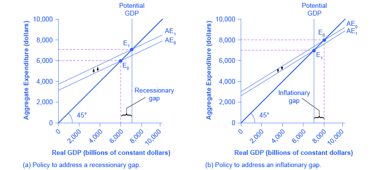
What might cause a recessionary gap? Anything that shifts the aggregate expenditure line down is a potential cause of recession, including a decline in consumption, a rise in savings, a fall in investment, a drop in government spending or a rise in taxes, or a fall in exports or a rise in imports. Moreover, an economy that is at equilibrium with a recessionary gap may just stay there and suffer high unemployment for a long time; remember, the meaning of equilibrium is that there is no particular adjustment of prices or quantities in the economy to chase the recession away.
The appropriate response to a recessionary gap is for the government to reduce taxes or increase spending so that the aggregate expenditure function shifts up from AE0 to AE1. When this shift occurs, the new equilibrium E1 now occurs at potential GDP as shown in Figure 1 (a).
Conversely, Figure 1 (b) shows a situation where the aggregate expenditure schedule (AE0) intersects the 45-degree line above potential GDP. The gap between the level of real GDP at the equilibrium E0 and potential GDP is called an inflationary gap. The inflationary gap also requires a bit of interpreting. After all, a naïve reading of the Keynesian cross diagram might suggest that if the aggregate expenditure function is just pushed up high enough, real GDP can be as large as desired—even doubling or tripling the potential GDP level of the economy. This implication is clearly wrong. An economy faces some supply-side limits on how much it can produce at a given time with its existing quantities of workers, physical and human capital, technology, and market institutions.
The inflationary gap should be interpreted, not as a literal prediction of how large real GDP will be, but as a statement of how much extra aggregate expenditure is in the economy beyond what is needed to reach potential GDP. An inflationary gap suggests that because the economy cannot produce enough goods and services to absorb this level of aggregate expenditures, the spending will instead cause an inflationary increase in the price level. In this way, even though changes in the price level do not appear explicitly in the Keynesian cross equation, the notion of inflation is implicit in the concept of the inflationary gap.
The appropriate Keynesian response to an inflationary gap is shown in Figure 1 (b). The original intersection of aggregate expenditure line AE0 and the 45-degree line occurs at $8,000, which is above the level of potential GDP at $7,000. If AE0 shifts down to AE1, so that the new equilibrium is at E1, then the economy will be at potential GDP without pressures for inflationary price increases. The government can achieve a downward shift in aggregate expenditure by increasing taxes on consumers or firms, or by reducing government expenditures.
The Multiplier Effect
The Keynesian policy prescription has one final twist. Assume that for a certain economy, the intersection of the aggregate expenditure function and the 45-degree line is at a GDP of 700, while the level of potential GDP for this economy is $800. By how much does government spending need to be increased so that the economy reaches the full employment GDP? The obvious answer might seem to be $800 – $700 = $100; so raise government spending by $100. But that answer is incorrect. A change of, for example, $100 in government expenditures will have an effect of more than $100 on the equilibrium level of real GDP. The reason is that a change in aggregate expenditures circles through the economy: households buy from firms, firms pay workers and suppliers, workers and suppliers buy goods from other firms, those firms pay their workers and suppliers, and so on. In this way, the original change in aggregate expenditures is actually spent more than once. This is called the multiplier effect: An initial increase in spending, cycles repeatedly through the economy and has a larger impact than the initial dollar amount spent.
How Does the Multiplier Work?
To understand how the multiplier effect works, return to the example in which the current equilibrium in the Keynesian cross diagram is a real GDP of $700, or $100 short of the $800 needed to be at full employment, potential GDP. If the government spends $100 to close this gap, someone in the economy receives that spending and can treat it as income. Assume that those who receive this income pay 30% in taxes, save 10% of after-tax income, spend 10% of total income on imports, and then spend the rest on domestically produced goods and services.
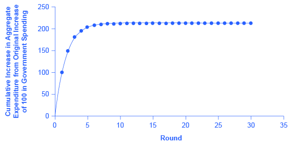
As shown in the calculations in Figure 2 and Table 1, out of the original $100 in government spending, $53 is left to spend on domestically produced goods and services. That $53 which was spent, becomes income to someone, somewhere in the economy. Those who receive that income also pay 30% in taxes, save 10% of after-tax income, and spend 10% of total income on imports, as shown in Figure 2, so that an additional $28.09 (that is, 0.53 × $53) is spent in the third round. The people who receive that income then pay taxes, save, and buy imports, and the amount spent in the fourth round is $14.89 (that is, 0.53 × $28.09).
| Original increase in aggregate expenditure from government spending | 100 |
| Which is income to people throughout the economy: Pay 30% in taxes. Save 10% of after-tax income. Spend 10% of income on imports. Second-round increase of… | 70 – 7 – 10 = 53 |
| Which is $53 of income to people through the economy: Pay 30% in taxes. Save 10% of after-tax income. Spend 10% of income on imports. Third-round increase of… | 37.1 – 3.71 – 5.3 = 28.09 |
| Which is $28.09 of income to people through the economy: Pay 30% in taxes. Save 10% of after-tax income. Spend 10% of income on imports. Fourth-round increase of… | 19.663 – 1.96633 – 2.809 = 14.89 |
Thus, over the first four rounds of aggregate expenditures, the impact of the original increase in government spending of $100 creates a rise in aggregate expenditures of $100 + $53 + $28.09 + $14.89 = $195.98. Figure 2 shows these total aggregate expenditures after these first four rounds, and then the figure shows the total aggregate expenditures after 30 rounds. The additional boost to aggregate expenditures is shrinking in each round of consumption. After about 10 rounds, the additional increments are very small indeed—nearly invisible to the naked eye. After 30 rounds, the additional increments in each round are so small that they have no practical consequence. After 30 rounds, the cumulative value of the initial boost in aggregate expenditure is approximately $213. Thus, the government spending increase of $100 eventually, after many cycles, produced an increase of $213 in aggregate expenditure and real GDP. In this example, the multiplier is $213/$100 = 2.13.
Calculating the Multiplier
Fortunately for everyone who is not carrying around a computer with a spreadsheet program to project the impact of an original increase in expenditures over 20, 50, or 100 rounds of spending, there is a formula for calculating the multiplier. And you’ve actually seen a simpler version of it (without taxes and imports) in the previous section.
[latex]\text{Spending Multiplier}=\frac{1}{1-MPC\times(1-\text{tax rate})+MPI}[/latex]
The data from Figure 2 and Table 1 is:
- Marginal Propensity to Save (MPS) = 10%
- Tax rate = 30%
- Marginal Propensity to Import (MPI) = 10%
The MPC is equal to 1 – MPS, or 0.9. Therefore, the spending multiplier is:
[latex]\begin{array}{rcl}\frac{1}{1-(0.9-(0.3)(0.9)-0.1)}=\frac{1}{0.47}=2.13\end{array}[/latex]
A change in spending of $100 multiplied by the spending multiplier of 2.13 is equal to a change in GDP of $213. Not coincidentally, this result is exactly what was calculated in Figure 2 after many rounds of expenditures cycling through the economy.
The size of the multiplier is determined by what proportion of the marginal dollar of income goes into taxes, saving, and imports. These three factors are known as “leakages,” because they determine how much demand “leaks out” in each round of the multiplier effect. If the leakages are relatively small, then each successive round of the multiplier effect will have larger amounts of demand, and the multiplier will be high. Conversely, if the leakages are relatively large, then any initial change in demand will diminish more quickly in the second, third, and later rounds, and the multiplier will be small. Changes in the size of the leakages—a change in the marginal propensity to save, the tax rate, or the marginal propensity to import—will change the size of the multiplier.
Calculating Keynesian Policy Interventions
Returning to the original question: How much should government spending be increased to produce a total increase in real GDP of $100? If the goal is to increase aggregate demand by $100, and the multiplier is 2.13, then the increase in government spending to achieve that goal would be $100/2.13 = $47. Government spending of approximately $47, when combined with a multiplier of 2.13 (which is, remember, based on the specific assumptions about tax, saving, and import rates), produces an overall increase in real GDP of $100, restoring the economy to potential GDP of $800, as Figure 3 shows.
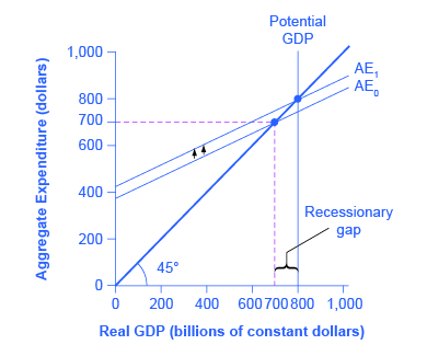
The multiplier effect is also visible on the Keynesian cross diagram. Figure 3 shows the example we have been discussing: a recessionary gap with an equilibrium of $700, potential GDP of $800, the slope of the aggregate expenditure function (AE0) determined by the assumptions that taxes are 30% of income, savings are 0.1 of after-tax income, and imports are 0.1 of before-tax income. At AE1, the aggregate expenditure function is moved up to reach potential GDP.
Now, compare the vertical shift upward in the aggregate expenditure function, which is $47, with the horizontal shift outward in real GDP, which is $100 (as these numbers were calculated earlier). The rise in real GDP is more than double the rise in the aggregate expenditure function. (Similarly, if you look back at Figure 1, you will see that the vertical movements in the aggregate expenditure functions are smaller than the change in equilibrium output that is produced on the horizontal axis. Again, this is the multiplier effect at work.) In this way, the power of the multiplier is apparent in the income–expenditure graph, as well as in the arithmetic calculation.
The multiplier does not just affect government spending, but applies to any change in the economy. Say that business confidence declines and investment falls off, or that the economy of a leading trading partner slows down so that export sales decline. These changes will reduce aggregate expenditures, and then will have an even larger effect on real GDP because of the multiplier effect. Read the following Clear It Up feature to learn how the multiplier effect can be applied to analyze the economic impact of professional sports.
How can the Multiplier be Used to Analyze the Economic Impact of Professional Sports?
Attracting professional sports teams and building sports stadiums to create jobs and stimulate business growth is an economic development strategy adopted by many communities throughout the United States. In his recent article, “Public Financing of Private Sports Stadiums,” James Joyner of Outside the Beltway looked at public financing for NFL teams. Joyner’s findings confirm the earlier work of John Siegfried of Vanderbilt University and Andrew Zimbalist of Smith College.
Siegfried and Zimbalist used the multiplier to analyze this issue. They considered the amount of taxes paid and dollars spent locally to see if there was a positive multiplier effect. Since most professional athletes and owners of sports teams are rich enough to owe a lot of taxes, let’s say that 40% of any marginal income they earn is paid in taxes. Because athletes are often high earners with short careers, let’s assume that they save one-third of their after-tax income.
However, many professional athletes do not live year-round in the city in which they play, so let’s say that one-half of the money that they do spend is spent outside the local area. One can think of spending outside a local economy, in this example, as the equivalent of imported goods for the national economy.
Now, consider the impact of money spent at local entertainment venues other than professional sports. While the owners of these other businesses may be comfortably middle-income, few of them are in the economic stratosphere of professional athletes. Because their incomes are lower, so are their taxes; say that they pay only 35% of their marginal income in taxes. They do not have the same ability, or need, to save as much as professional athletes, so let’s assume their MPC is just 0.8. Finally, because more of them live locally, they will spend a higher proportion of their income on local goods—say, 65%.
If these general assumptions hold true, then money spent on professional sports will have less local economic impact than money spent on other forms of entertainment. For professional athletes, out of a dollar earned, 40 cents goes to taxes, leaving 60 cents. Of that 60 cents, one-third is saved, leaving 40 cents, and half is spent outside the area, leaving 20 cents. Only 20 cents of each dollar is cycled into the local economy in the first round. For locally-owned entertainment, out of a dollar earned, 35 cents goes to taxes, leaving 65 cents. Of the rest, 20% is saved, leaving 52 cents, and of that amount, 65% is spent in the local area, so that 33.8 cents of each dollar of income is recycled into the local economy.
Siegfried and Zimbalist make the plausible argument that, within their household budgets, people have a fixed amount to spend on entertainment. If this assumption holds true, then money spent attending professional sports events is money that was not spent on other entertainment options in a given metropolitan area. Since the multiplier is lower for professional sports than for other local entertainment options, the arrival of professional sports to a city would reallocate entertainment spending in a way that causes the local economy to shrink, rather than to grow. Thus, their findings seem to confirm what Joyner reports and what newspapers across the country are reporting. A quick Internet search for “economic impact of sports” will yield numerous reports questioning this economic development strategy.
Multiplier Tradeoffs: Stability versus the Power of Macroeconomic Policy
Is an economy healthier with a high multiplier or a low one? With a high multiplier, any change in aggregate demand will tend to be substantially magnified, and so the economy will be more unstable. With a low multiplier, by contrast, changes in aggregate demand will not be multiplied much, so the economy will tend to be more stable.
However, with a low multiplier, government policy changes in taxes or spending will tend to have less impact on the equilibrium level of real output. With a higher multiplier, government policies to raise or reduce aggregate expenditures will have a larger effect. Thus, a low multiplier means a more stable economy, but also weaker government macroeconomic policy, while a high multiplier means a more volatile economy, but also an economy in which government macroeconomic policy is more powerful.
equilibrium at a level of output below potential GDP
equilibrium at a level of output above potential GDP
