
11.2 – The Building Blocks of Neoclassical Analysis
Learning Objectives
By the end of this section, you will be able to:
- Explain the importance of Say’s Law and long run aggregate supply curve
- Analyze the role of flexible prices
- Analyze the tendency toward full employment through flexible wages in the labor market
- Apply supply and demand models to unemployment and wages
- Explain how the loanable funds market models the financial sector
- Explain how the orthodox economists understand thrift to be an important source for economic growth
- Interpret a neoclassical model of aggregate demand and aggregate supply
The neoclassical perspective on macroeconomics holds that, in the long run, the economy will fluctuate around its potential GDP and its natural rate of unemployment. This chapter begins with two building blocks of neoclassical economics: (1) potential GDP determines the economy’s size and (2) wages and prices will adjust in a flexible manner so that the economy will adjust back to its potential GDP level of output. The key policy implication is this: The government should focus more on long-term growth and on controlling inflation than on worrying about recession or cyclical unemployment. Let’s consider the two neoclassical building blocks in turn, and how we can embody them in the aggregate demand/aggregate supply model.
Say’s Law and the Importance of Potential GDP in the Long Run
Those economists who emphasize the role of supply in the macroeconomy often refer to the work of a famous early nineteenth century French economist named Jean-Baptiste Say (1767–1832). Say’s law is: “Supply creates its own demand.” As a matter of historical accuracy, it seems clear that Say never actually wrote down this law and that it oversimplifies his beliefs, but the law lives on as useful shorthand for summarizing a point of view.
The intuition behind Say’s law is that each time a good or service is produced and sold, it generates income that is earned for someone: a worker, a manager, an owner, or those who are workers, managers, and owners at firms that supply inputs along the chain of production. Similar to the discussion in the earlier Chapter: The Macroeconomic Perspective in which the National Income approach to measuring GDP is described… The forces of supply and demand in individual markets will cause prices to rise and fall. The bottom line remains, however, that every sale represents income to someone, and so, Say’s law argues, a given value of supply must create an equivalent value of demand somewhere else in the economy. Modern economists who generally subscribe to the Say’s law view on the importance of supply for determining the size of the macroeconomy are called orthodox economists.
If supply always creates exactly enough demand at the macroeconomic level, then (as Say himself recognized) it is hard to understand why periods of recession and high unemployment should ever occur. To be sure, even if total supply always creates an equal amount of total demand, the economy could still experience a situation of some firms earning profits while other firms suffer losses. Nevertheless, a recession is not a situation where all business failures are exactly counterbalanced by an offsetting number of successes. A recession is a situation in which the economy as a whole is shrinking in size, business failures outnumber the remaining success stories, and many firms end up suffering losses and laying off workers.
Among orthodox economists, short-run fluctuations aside, Say’s law stipulation that supply creates its own demand is perceived as an appropriate approximation for the long run. Over periods of some years or decades, as the productive power of an economy to supply goods and services increases, total demand in the economy grows at roughly the same pace. However, over shorter time horizons of a few months or even years, recessions or even depressions occur in which firms, as a group, seem to face a lack of demand for their products.
Orthodox economists believe that over the long run the level of potential GDP determines the size of real GDP. When economists refer to “potential GDP” they are referring to that level of output that an economy can achieve when all resources (land, labor, capital, and entrepreneurial ability) are fully employed. While the unemployment rate in labor markets will never be zero, full employment in the labor market refers to zero cyclical unemployment. There will still be some level of unemployment due to frictional or structural unemployment, but when the economy is operating with zero cyclical unemployment, economists say that the economy is at the natural rate of unemployment or at full employment.
Economists benchmark actual or real GDP against the potential GDP to determine how well the economy is performing. As explained in Economic Growth, we can explain GDP growth by increased investment in physical capital and human capital per person as well as advances in technology. Physical capital per person refers to the amount and kind of machinery and equipment available to help people get work done. Compare, for example, your productivity in typing a term paper on a typewriter to working on your laptop with word processing software. Clearly, you will be able to be more productive using word processing software. The technology and level of capital of your laptop and software has increased your productivity. More broadly, the development of GPS technology and Universal Product Codes (those barcodes on every product we buy) has made it much easier for firms to track shipments, tabulate inventories, and sell and distribute products. These two technological innovations, and many others, have increased a nation’s ability to produce goods and services for a given population. Likewise, increasing human capital involves increasing levels of knowledge, education, and skill sets per person through vocational or higher education. Physical and human capital improvements with technological advances will increase overall productivity and, thus, GDP.
To see how these improvements have increased productivity and output at the national level, we should examine evidence from the United States. The United States experienced significant growth in the twentieth century due to phenomenal changes in infrastructure, equipment, and technological improvements in physical capital and human capital. The population more than tripled in the twentieth century, from 76 million in 1900 to over 300 million in 2016. The human capital of modern workers is far higher today because the education and skills of workers have risen dramatically. In 1900, only about one-eighth of the U.S. population had completed high school and just one person in 40 had completed a four-year college degree. By 2010, more than 87% of Americans had a high school degree and over 29% had a four-year college degree as well. In 2014, 40% of working-age Americans had a four-year college degree.
The average amount of physical capital per worker has grown dramatically as well. The technology available to modern workers is extraordinarily better than a century ago: cars, airplanes, electrical machinery, smartphones, computers, chemical and biological advances, materials science, health care—the list of technological advances could run on and on. More workers, higher skill levels, larger amounts of physical capital per worker, and amazingly better technology, and potential GDP for the U.S. economy has clearly increased a great deal since 1900.
This growth has fallen below its potential GDP and, at times, has exceeded its potential. For example from 2008 to 2009, the U.S. economy tumbled into recession and remains below its potential. At other times, like in the late 1990s, the economy ran at potential GDP—or even slightly ahead. Figure 1 shows the actual data for the increase in real GDP since 1960. The slightly smoother line shows the potential GDP since 1960 as estimated by the nonpartisan Congressional Budget Office. Most economic recessions and upswings are times when the economy is 1–3% below or above potential GDP in a given year. Clearly, short-run fluctuations around potential GDP do exist, but over the long run, the upward trend of potential GDP determines the size of the economy.
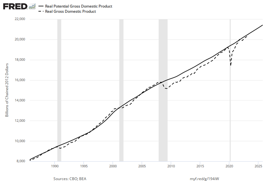
Figure 1. Potential and Actual GDP (in 2009 Dollars) Actual GDP falls below potential GDP during and after recessions, like the recessions of 1990–91, 2001, and 2008–2009 and continued well below potential GDP after the Great Recession. In other cases, actual GDP can be above potential GDP for a time, as in the late 1990s.
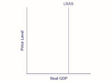
In the aggregate demand/aggregate supply model, we show potential GDP as a vertical line. Neoclassical economists who focus on potential GDP as the primary determinant of real GDP argue that the long-run aggregate supply curve is located at potential GDP—that is, we draw the long-run aggregate supply curve as a vertical line at the level of potential GDP, as Figure 2 shows. A vertical LRAS curve means that the level of aggregate supply (or potential GDP) will determine the economy’s real GDP, regardless of the level of aggregate demand. Over time, increases in the quantity and quality of physical capital, increases in human capital, and technological advancements shift potential GDP and the vertical LRAS curve gradually to the right. Economists often describe this gradual increase in an economy’s potential GDP as a nation’s long-term economic growth.
The Loanable Funds Market and Economic Growth in Neoclassical Economics
Given Say’s law, neoclassical economists believe that a vertical LRAS curve means that the level of aggregate supply (or potential GDP) will determine the economy’s real GDP, regardless of the level of aggregate demand. However, there is one potential problem: what happens when the households that participated in creating the output (as workers, landlords, capitalists, and so on), decide not to use their income to purchase that output? That is, what happens when income is saved?
The solution to this problem in the neoclassical framework is the loanable funds market. Through this market, household savings are channeled into business loans for investment. As a result, any income not spent (that is, saved) becomes investment, which of course is a type of spending. All of this is really just another way of ensuring that in this model Say’s Law holds: supply creates its own demand, and if there is less supply than is possible (at full employment), or insufficient demand to purchase that supply, then price adjustments will correct the imbalances.
The Loanable Funds Market
In the loanable funds market, the price is the interest rate and the thing being exchanged is money. Households act as suppliers of money through saving, and they will supply a larger quantity of money (that is, they will save more) as the interest rate increases. This should be intuitive: the interest rate is the return (or reward) you earn for saving your money; the higher the interest rate, the more inclined you will be to save.
Businesses, in turn, are the demanders in the loanable funds market. Here, businesses are borrowing the money households save so that they can make real investments–for instance, buying a new fleet of delivery vans or upgrading the office computers’ software. As is the usual case, demand declines with price. For the loanable funds market, this means that, the lower the interest rate, the greater the amount of money businesses will want to borrow, since the interest rate is the cost of taking out the loan.
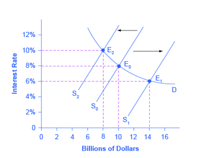
Looking to the figure below, we can see that, when the supply of loanable funds is at S0, the equilibrium (E0) occurs at an 8% interest rate and a quantity of funds loaned and borrowed of $10 billion. This suggests that, at an 8% interest rate, households will be saving a total of $10 billion. By definition, this means that households aren’t spending $10 billion of their income, which is a problem for Say’s Law: output is $10 billion higher than household spending. But, of course, at an 8% interest rate, businesses will be borrowing $10 billion and, most importantly, spending that money on real investment.
Hence, the problem of saving is solved: so long as the interest rate adjusts to equilibrium in the loanable funds market, any income not spent (that is, money saved) will ultimately become spending through investment. In a sense, this is an extension of Say’s Law: supply creates its own demand, but money saved is supply (production) that created income that didn’t create demand (spending). Not to worry, though, because saving in the orthodox framework is its own kind of supply (to the loanable funds market), which becomes spending just the same.
The Power of Thrift
The loanable funds market isn’t just a clever solution to the problem of saving and Say’s Law, it’s the basic way that orthodox economists understand the financial sector in general. While you’ll learn more about the complexity of the financial sector and how economists understand it in later chapters, it is worth looking at one important conclusion derived from the loanable funds model. Namely, this framework suggests that saving is the fundamental engine for economic growth.
The importance of saving for growth will be clear once we recognize that investment, in machines, research & development, software upgrades, and so on, is what increases productivity, which in turn is what spurs growth in general. And, since in the loanable funds market, investment is financed through loans which are funded with households’ savings, then it makes sense to see saving as the ultimate source of economic growth.
We can see this process working in the graph above. An increase in the thriftiness–that is, the desire to save–among households will shift the supply of loanable funds to the right from the original supply curve (S0) to S1. This will lead to an equilibrium (E1) with a lower 6% interest rate and a quantity $14 billion in loaned funds. At this lower interest rate, the cost of borrowing for investment is lower, which means more businesses will be willing to make greater investments.
Conversely, if households desire to save less and spend more of their income, moving the loanable funds supply curve, say, from S0 to S2. the result would be a higher interest rate, leading to lower levels of investment. In this scenario, households are enjoying more of the fruits of their labor today, through current consumption, but at the expense of investing in productivity growth for the future.
The Labor Market and the Tendency toward Full Employment
We have seen that unemployment varies across times and places, but that, at least according to orthodox economics, capitalist economies should tend toward the natural rate of unemployment in the long run. Below, you’ll read about how this tendency is supposed to work and why, according to orthodox theory, it often doesn’t.
Earlier in this chapter, you learned that the economy should, in the long run, reach an equilibrium level of output at potential GDP. This occurs at the intersection of the aggregate demand (AD) and the long-run aggregate supply (LRAS) curves and is consistent with full employment (or the natural rate of unemployment). The labor market model is one way of understanding how, at least in the absence of sticky prices, this would occur. Recall that higher prices for the things firms sell, relative to input costs for producing those things, will induce firms to produce and sell more output. It follows then that lower input costs, relative to prices, would also lead firms to hire more workers and produce more output.
This suggests that we can understand the long run tendency for capitalist economies to fully employ their resources (that is, inputs like labor) in terms of the prices of those inputs. Below, we’ll look at how the competitive market for labor should ensure full employment. (Note, however, that these arguments should apply to any of the real resources that firms use as inputs to produce the goods and services that make up GDP.)
The Labor Market
Neoclassical economists understand the processes of firms hiring and workers working for pay by using the standard supply-and-demand model. Demand represents the firms paying for workers’ time and effort, and supply represents the workers supplying their labor. The wage rate, then, is the price of the labor, and if the labor market is in equilibrium (at a wage rate of We in the figure below), then the quantity of work that workers want to do (or supply) will be equal to the quantity that firms want to hire (or demand).
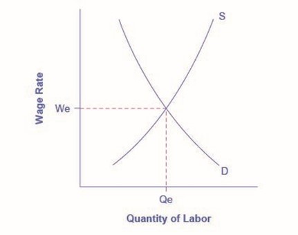
One possibility for any observed unemployment is that people who are unemployed are those who are not willing to work at the current equilibrium wage, say $10 an hour, but would be willing to work at a higher wage, like $20 per hour. The monthly Current Population Survey would count these people as unemployed, because they say they are ready and looking for work (at $20 per hour). However, from an economist’s perspective, these people are choosing to be unemployed, so they’re ignored in terms of the tendency to full employment.
Hence, in general, all orthodox economists, and particularly neoclassical economists, argue that the key to full employment is flexible wages. As in the figure below, unemployment is defined as an excess supply of labor, relative to demand for it from firms, and the supply-and-demand model tells us that this is resolved through a drop in the wage rate. Of course, this was implied by the idea that firms will produce more when the prices of the things they sell go up relative to the costs of producing those things. If we treat the wage rate in the figure above as the real (that is, inflation-adjusted) wage rate, then a decrease in how much firms pay their workers is the same as an increase in prices (which corresponds to a decrease in the real, inflation-adjusted wage rate).
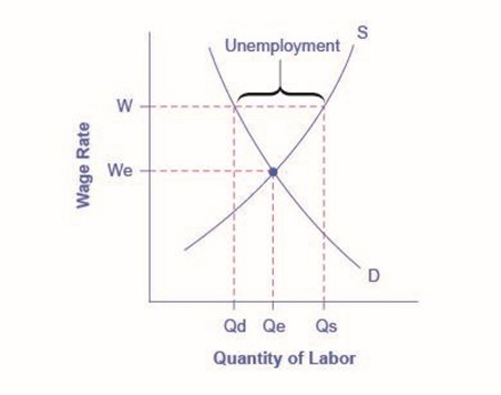
It follows, then, that persistent involuntary unemployment that cannot be attributed to structural or frictional causes must be due a breakdown in the price mechanism itself. That is, unemployment must be a result of something keeping the real wage rate from falling. Orthodox economists often refer to these situations as wages being ‘sticky downward.’
The Role of Flexible Prices
How does the macroeconomy adjust back to its level of potential GDP in the long run? What if aggregate demand increases or decreases? Economists base the neoclassical view of how the macroeconomy adjusts on the insight that even if wages and prices are “sticky”, or slow to change, in the short run, they are flexible over time. To understand this better, let’s follow the connections from the short-run to the long-run macroeconomic equilibrium.
The aggregate demand and aggregate supply diagram in [link] shows two aggregate supply curves. We draw the original upward sloping aggregate supply curve (SRAS0) is a short-run or AS curve. The vertical aggregate supply curve (LRASn) is the long-run or neoclassical AS curve, which is located at potential GDP. The original aggregate demand curve, labeled AD0, so that the original equilibrium occurs at point E0, at which point the economy is producing at its potential GDP.
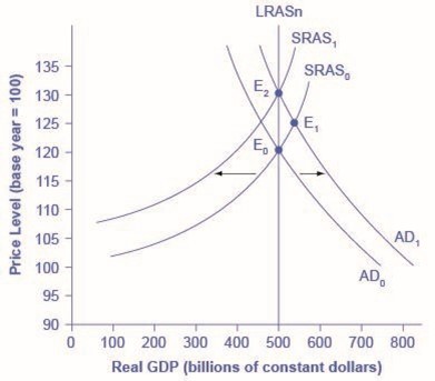
Now, imagine that some economic event boosts aggregate demand: perhaps a surge of export sales or a rise in business confidence that leads to more investment, perhaps a policy decision like higher government spending, or perhaps a tax cut that leads to additional aggregate demand. The short-run analysis is that the rise in aggregate demand will shift the aggregate demand curve out to the right, from AD0 to AD1, leading to a new equilibrium at point E1 with higher output, lower unemployment, and pressure for an inflationary rise in the price level.
In the neoclassical analysis, however, the chain of economic events is just beginning. As economic output rises above potential GDP, the level of unemployment falls. The economy is now above full employment and there is a labor shortage. Eager employers are trying to bid workers away from other companies and to encourage their current workers to exert more effort and to work longer hours. This high demand for labor will drive up wages. Most employers review their workers salaries only once or twice a year, and so it will take time before the higher wages filter through the economy. As wages do rise, it will mean a leftward shift in the short-run aggregate supply curve back to SRAS1, because the price of a major input to production has increased. The economy moves to a new equilibrium (E2). The new equilibrium has the same level of real GDP as did the original equilibrium (E0), but there has been an inflationary increase in the price level.
This description of the short-run shift from E0 to E1 and the long-run shift from E1 to E2 is a step-by-step way of making a simple point: the economy cannot sustain production above its potential GDP in the long run. An economy may produce above its level of potential GDP in the short run, under pressure from a surge in aggregate demand. Over the long run, however, that surge in aggregate demand ends up as an increase in the price level, not as a rise in output.
The rebound of the economy back to potential GDP also works in response to a shift to the left in aggregate demand. Figure 4 again starts with two aggregate supply curves, with SRAS0 showing the original upward sloping short-run AS curve and LRASn showing the vertical long-run neoclassical aggregate supply curve. A decrease in aggregate demand—for example, because of a decline in consumer confidence that leads to less consumption and more saving—causes the original aggregate demand curve AD0 to shift back to AD1. The shift from the original equilibrium (E0) to the new equilibrium (E1) results in a decline in output. The economy is now below full employment and there is a surplus of labor. As output falls below potential GDP, unemployment rises. While a lower price level (i.e., deflation) is rare in the United States, it does happen occasionally during very weak periods of economic activity. For practical purposes, we might consider a lower price level in the AD–AS model as indicative of disinflation, which is a decline in the inflation rate. Thus, the long-run aggregate supply curve LRASn, which is vertical at the level of potential GDP, ultimately determines this economy’s real GDP.
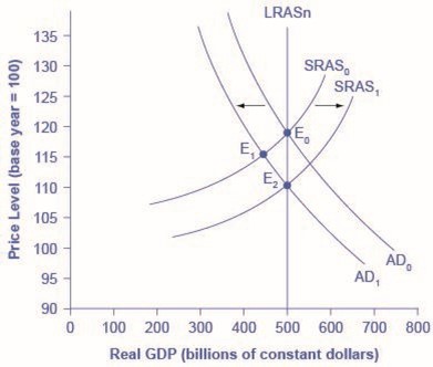
Again, from the neoclassical perspective, this scenario is only the beginning of the chain of events. The higher level of unemployment means more workers looking for jobs. As a result, employers can hold down on pay increases—or perhaps even replace some of their higher-paid workers with unemployed people willing to accept a lower wage. As wages stagnate or fall, this decline in the price of a key input means that the short-run aggregate supply curve shifts to the right from its original position (SRAS0 to SRAS1). The overall impact in the long run, as the macroeconomic equilibrium shifts from E0 to E1 to E2, is that the level of output returns to potential GDP, where it started. There is, however, downward pressure on the price level. Thus, in the neoclassical view, changes in aggregate demand can have a short-run impact on output and on unemployment—but only a short-run impact. In the long run, when wages and prices are flexible, potential GDP and aggregate supply determine real GDP’s size.
How Fast Is the Speed of Macroeconomic Adjustment?
How long does it take for wages and prices to adjust, and for the economy to rebound to its potential GDP? Within orthodox economics the subject has warranted some debate, while across the sweep of economic ideas, including heterodox perspectives, the subject is highly contentious.
One subset of neoclassical economists holds that wage and price adjustment in the macroeconomy might be quite rapid. The theory of rational expectations holds that people form the most accurate possible expectations about the future that they can, using all information available to them. In an economy where most people have rational expectations, economic adjustments will happen very quickly, such that price adjustments appear as an immediate movement along the vertical long run aggregate supply curve.
For example, when a shift in aggregate demand occurs, people and businesses with rational expectations will know that its impact on output and employment will be temporary, while its impact on the price level will be permanent. If firms and workers perceive the outcome of the process in advance, and if all firms and workers know that everyone else is perceiving the process in the same way, then they have no incentive to go through an extended series of short-run scenarios, like a firm first hiring more people when aggregate demand shifts out and then firing those same people when aggregate supply shifts back. Instead, everyone will recognize where this process is heading—toward a change in the price level—and then will act on that expectation. In this scenario, the expected long-run change in the price level may happen very quickly, without a drawn-out zigzag of output and employment first moving one way and then the other.
Prior to the advent of the theory of rational expectations, another wage and price assumption, originally presented by Milton Friedman, as part of the monetarist argument, argued that people and firms act with adaptive expectations: they look at past experience and gradually adapt their beliefs and behavior as circumstances change, but are not perfect synthesizers of information and accurate predictors of the future in the sense of rational expectations theory. If most people and businesses have some form of adaptive expectations, then the adjustment from the short run and long run will be traced out in incremental steps that occur over time.
Troubling for neoclassical economics, the empirical evidence on the speed of macroeconomic adjustment of prices and wages is not clear-cut. The speed of macroeconomic adjustment may vary among different countries and time periods. Neoclassical economics is prone to guess that the initial short-run effect of a shift in aggregate demand might last two to five years, before the adjustments in wages and prices cause the economy to adjust back to the neoclassical perception of the long run. As a result of these discrepancies another, more demand driven strand of orthodox economics has developed. New-Keynesian analysis, the subject of the next section, suggests that waiting on an uncertain long run is unnecessary as well as potentially harmful and thus there is a case for using government policy to more quickly address periods of perceived sticky wages and prices.
Summary
The neoclassical perspective argues that, in the long run, the economy will adjust back to its potential GDP level of output through flexible price levels. Thus, the neoclassical perspective views the long-run AS curve as vertical. A rational expectations perspective argues that people have excellent information about economic events and how the economy works and that, as a result, price and other economic adjustments will happen very quickly. In adaptive expectations theory, people have limited information about economic information and how the economy works, and so price and other economic adjustments can be slow.
"supply creates its own demand"
a significant decline in national output
GDP adjusted for changes in prices over time
the maximum quantity that an economy can produce given full employment of its existing levels of labor, physical capital, technology, and institutions
the accumulated skills and education of workers
the total quantity of output (i.e. real GDP) firms will produce and sell
the amount of total spending on domestic goods and services in an economy
the market in which households sell their labor as workers to business firms or other employers
