In the previous chapter we considered a hypothetical economy that produces only two goods: corn and steel. Specifically:

[latex]20 \text{ corn} + 80 \text{ steel} → 420 \text{ corn} \\ 144 \text{ corn} + 4 \text{ steel} → 84 \text{ steel}[/latex]

In that model we assumed that the steel sector produced just enough steel to replace the steel used up as inputs in both sectors. In the above model you can see that the two sectors, corn and steel, use 84 tons of steel in total, and the steel sector produces exactly that amount. We also said that the corn sector produced a surplus–that is, more corn than would be needed in the next year to continue producing. Notice that this surplus comes out to 256 tons of corn, which is the 420 tons of corn produced (right-hand side of the first equation) minus the 164 tons of corn used up in production (adding the first terms of both equations). As we saw in the previous chapter, this yielded businesses in both sectors a profit rate of 61.54%.

To keep things simple, we assumed previously that (1) the surplus was a given, fixed quantity, and (2) the entire surplus was accumulated by business owners in the form of profits. Below we’ll drop each of these assumptions to answer our two questions of interest: what determines how big the surplus is, and how is the surplus distributed? Let’s start with the first question.

In our simple economy, we have 84 tons of steel being produced–just enough to continue production in the future–and 420 tons of corn being produced, which leaves a surplus of 256 tons. But why not more? That is, what prevents the economy from producing a greater surplus than this?

The obvious answer might be that there aren’t enough workers, or land, or other resources to allow for more output than this. And this may or may not be the case for a particular economy in a particular period. But remember, from the heterodox perspective a capitalist economy will not necessarily–or even normally–operate at a level of aggregate output in which its resources are fully employed–it’s possible, but probably not typical. Instead, underemployment of workers and underutilization of other resources is more likely. So if the economy is in that situation, where more could be produced than currently is being produced, what might move output up?

The heterodox perspective, following the arguments of Keynes and colleagues, approaches this question from the demand side (see Chapter “The Keynesian Perspective”). That is, total output in the economy follows from the total spending being done. In our simple model, the spending can be broken down into the following:

1. The spending by workers on food (corn). But for the time being we’re assuming workers only get a subsistence income, and so this spending is really just part of the corn quantities in each of the sectors. To say that they receive a subsistence income is to say that workers are only being paid the bear minimum necessary for their survival. We’ll drop this assumption later.
2. Investment outlays, which is to say the corn and steel necessary to produce the corn in the corn sector and the steel in the steel sector.
3. Spending by business owners and managers–that is, in essence, what they would like to do with the surplus.

Now, since we’ve said that workers are paid only a subsistence income, then by assumption they can’t spend more than the bare minimum necessary to survive. Similarly, since the relative input requirements–that is, how much corn and steel is necessary to produce a ton of corn or a ton of steel–are technologically determined, investment outlays have to increase or decrease in a certain proportion to each other. Which brings us to the basic source of the spending decision that drives all the other spending and ultimately the level of output: spending by business owners/managers. In short, if business owners desire to create a larger surplus, they will do so by increasing their investment outlays (in the fixed proportions given by technology) and, provided the additional unemployed resources are available to do so, the surplus will grow. That is, of the three types of spending listed above, it’s the third that’s really capable of driving up output in general.

Let’s return to our hypothetical economy to see how this works. Suppose that last year the economy produced the surplus of 256 tons of corn that we’ve been working with previously. Then suppose that this year business owners have decided to increase their investment outlays so that a greater surplus can be produced. Perhaps they’re planning for a feast. Or perhaps corn companies intend to expand production into fallow land next year, which would of course require investments for more corn seed this year. Or maybe something more…interesting is planned, like a corn palace.

Regardless of the reasons the managers or owners of these companies may have, the impact is the same: a desire to increase surplus output requires more spending on investment–that is, on outlays for inputs into corn production. Hypothetically, we’ll say that the desire is to increase corn production from a total of 420 tons of corn to 930 tons, an increase of 510 tons.

Now, not all of that 510 tons of corn will be surplus, of course. The reason is that it takes more corn (to feed the agricultural workers as well as to seed the crop) to grow more corn. Let’s say that to grow 930 tons of corn it takes as an input 30 tons of corn. So we’re producing 510 more tons of corn, but it’s taking 10 more tons of corn to do so. Then the net increase in corn surplus, so far, is only 500 tons.

But to grow this greater amount of corn it also takes more steel to craft the farming implements (plows and so on). Let’s say that the corn sector is now looking at 150 tons of steel to grow its larger yield, an increase of 70 tons.

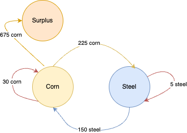
It’s just a bit more complicated than that, though, because, if the corn sector needs more steel, then the steel sector needs to be able to produce more steel. And for the steel sector to produce more steel, it will need as inputs both more corn and more steel. Specifically, in this hypothetical economy we’ll say that the steel sector will need 225 tons of corn and 5 tons of steel to produce 155 tons of steel. Since the corn sector needs 150 tons of steel, and the steel sector will need another 5 tons, then the 155 ton output in the steel sector will be just enough to keep it viable into the future.

Note as well that the steel sector now requires another 81 tons of corn (it originally needed 144 tons to feed its workers, but now it needs 224 tons), so our net surplus of corn drops further, from 500 to 419 tons. The economy was producing 256 tons of surplus corn; now it’s producing 675 tons of surplus corn. Presumably that’s still enough to build the corn palace we’re working on–the purpose of the increase in corn surplus.

If all of the numbers in the previous paragraphs were hard to follow, don’t worry, the following summarizes the numbers we’ve been looking at. Once again, we’ve got two sectors (first the corn sector, next steel) using both corn and steel to produce their products.

[latex]30 \text{ corn} + 150 \text{ steel} → 930 \text{ corn} \\ 225 \text{ corn} + 5 \text{ steel} → 155 \text{ steel}[/latex]

To be sure that you have followed the preceding text, you should compare these numbers to those presented at the beginning of this chapter (which are the same as in the previous chapter). Make sure you understand not just how the numbers have increased but also why, beginning with the increase in corn output (from 420 to 930 tons).

We’ll skip the calculations here (but see the section “A Corn Model Example” in the previous chapter) and go right to the relative prices, profits, and profit rates for each sector. By design–to keep the example simple–we’ve picked the numbers in our hypothetical economy so that the relative prices of steel and corn haven’t changed. Steel should still be selling at three times the price of corn in order to ensure that (1) both sectors can afford to buy the inputs they need from the other sector, and (2) the business owners in both sectors enjoy the same rate of profit.

As in the previous chapter, we’ll assume that corn sells for $10 a ton, and therefore steel must sell for $30 a ton. In this case, the corn sector’s profits (revenues minus expenses) are 930 tons of corn times $10 per ton, less 30 tons of corn at $10 per ton and 150 tons of steel at $30 per ton:

[latex]\text{Profit}_\text{corn} = $9,300 - $300 - $4,500 = $4,500[/latex]

Considering profit as a percentage over investment outlays–that is, the money spent on corn and steel in the corn sector–, we get:

[latex]\text{Rate of profit}_\text{corn} = \frac{$4,500}{$300 + $4,500} = \frac{$4,500}{$4,800} = 0.9375 = 93.75\%[/latex]

That’s a healthy profit margin. Let’s see how the steel sector did. Their revenues are 155 tons of steel produced times $30 per ton, which comes to $4,650. Profits, then, are revenues of $4,650 less 225 tons of corn at $10 per ton and 5 tons of steel at $30 per ton:

[latex]\text{Profit}_\text{steel} = $4,650 - $2,250 - $150 = $2,250[/latex]

And the rate of profit:

[latex]\text{Rate of profit}_\text{steel} = \frac{$2,250}{$2,250 + $150} = \frac{$2,250}{$2,400} = 0.9375 = 93.75\%[/latex]

It’s time to compare. With the original numbers, the economy was producing a surplus of 256 tons of corn; it’s now producing a surplus of 675 tons. The prices haven’t changed; steel still sells for three times the price of corn. And the return on investment–the rate of profit–is still equal between the two sectors, so it’s no more profitable to buy shares of corn-producing businesses than steel-producing businesses.

But, importantly, the profit rate itself has changed. Businesses in both sectors are now earning a 93.75% rate of profit, whereas they were only earning 61.54% before. Indeed, outright profits (in dollar terms) are higher. The corn producers are bringing in $4,500 on the whole, versus only $1,600 before; and steel companies are collectively pulling $2,250, when they were only getting $960 before. These are apparently good times for businesses in both sectors. We should review what happened to bring on such prosperity.

In the beginning, managers of the corn companies saw a reason to produce more corn–perhaps to keep up with the proliferating corn palaces across the region (“Why should Mitchell, South Dakota get a corn palace and not we here in Plankinton?”). To get this done, the corn producers had to increase their outlays–more corn to seed the land and feed the workers, and more steel for tools. This of course meant more spending in the steel sector as well, to feed their workers, to keep up with demand from the corn sector, and to maintain the greater productive capacity in the steel sector itself.

Hence, in general, business investment increased. With greater business spending came the intended larger surplus of corn (since there were unemployed resources to work with); and since we’re so far maintaining that the entire surplus goes to profits, the larger surplus means of course greater profits. This means, as well, a higher rate of profits, which is simply calculated as the (much higher) profits over the (somewhat higher) outlays.

The takeaway is simple enough: assuming there are unemployed resources to be brought into the production process (and there usually are), businesses themselves ultimately decide how much will be produced and how much profits they will make. They do so when they decide how much to invest. Again, following Keynes’ Law, spending ultimately dictates output and income.

Of course, in the real world businesses don’t actually make collective decisions about total investment; and, in a way, this is one of the major problems with capitalism. That is, because total investment is the core driver of private sector spending, and because that spending ultimately determines how much is produced and how much of our resources are employed, and because total investment is not collectively determined, then there’s nothing to ensure full employment–not in the private sector anyway. Sure, it’s possible that the race to construct mighty palaces of corn is sufficiently vigorous to put to work everyone willing and able to do so. But it’s also possible, and much more likely, that most of the time businesses simply won’t be so inclined to make the investments necessary to keep output up and unemployment down–and there’s nothing about capitalism that says they have to.

Glossary

subsistence income

the bear minimum necessary for their survival