
12.3 – A Heterodox Macroeconomic Perspective
Learning Objectives
By the end of this section, you will be able to:
- Explain the conditions of the Great Depression.
- Explain the limitations of orthodox economics in comparison to the Great Depression
- Analyze the influence of aggregate demand on the macroeconomy.
- Analyze the destabilizing aspects of the orthodox wage and price adjustment story.
The measure of any theory is its effectiveness in explaining real world conditions and events. In this regard, neither the neoclassical perspective nor the New Keynesian perspective can explain the events of the Great Depression (the very event responsible for the splitting of economics into two branches, microeconomics and macroeconomics):
| Year | Unemployment Rate | Change in GDP | Change in Price Level |
| 1929 | 3.2% | – | 0.6% |
| 1930 | 8.7% | -8.5% | -6.4% |
| 1931 | 15.9% | -6.4% | -9.3% |
| 1932 | 23.6% | -12.9% | -10.3% |
| 1933 | 24.9% | -1.2% | 0.8% |
The data in the table above depicts three events unfolding simultaneously, 1) declining production, 2) declining employment, and 3) declining overall price level. For all intents and purposes, these three conditions cannot and should not simultaneously occur according to either the neoclassical perspective or the New Keynesian perspective.
Consider, according to the orthodox perspective, the declining overall price level should return the economy to the full employment level of production. Assuming that a fully employed economy is one in which the unemployment rate is 4% or less, in Table 1 the decline in the overall price level is definitely not restoring full employment.
Alternatively, consider the data in contrast to the New Keynesian story. The New Keynesian model argues that sticky prices could conceivably explain a less than full employment circumstance. However, in Table 1, the unemployment rate increases even as flexible, certainly not sticky, prices coincide with less than full employment and price driven deflation.
Most significantly, contrary to both the neoclassical and New Keynesian perspectives, price flexibility during the Great Depression did not restore full employment! Simultaneously, nor does price stickiness seem to cause persistent unemployment. Clearly, orthodox economics does not have a firm theoretical grasp on the events associated with the Great Depression. To correctly account for the events of the Great Depression, another theoretical perspective is necessary.
In the next section we will explore “original” Keynesian thought. Deviating from both the neoclassical perspective as well as the New Keynesian perspective, the original Keynesian perspective will argue that the flexibility of wages and prices will worsen, as opposed to correct, economic instability.
Turning the Bowl Upside Down: A Heterodox Interpretation of Price Adjustments.
The orthodox economic story told above is the same story that was extolled by the neoclassical school of economists during the Great Depression. Entrenched ideas are hard to shake. In the preface to The General Theory, Keynes summed up this condition, “The difficulty lies, not in the new ideas, but in escaping from the old ones, which ramify, for those brought up as most of us have been, into every corner of our minds.” Ironically, at least for a period of time in the post-World War II era, Keynes’ arguments were successful in escaping from the ideas of the neoclassicals. Keynes’ escape, however, proved only to be temporary. Clearly the old ideas of the neoclassicals began reappearing shortly after World War 2 with the neoclassical synthesis (a neoclassical/New Keynesian hybrid) of the late 1940s and, ultimately, in the 1970s with the ongoing development of the neoclassical paradigm.
The orthodox understanding of price adjustments is fundamentally different from a heterodox perspective. Utilizing Keynes’ The General Theory of Employment, Interest, and Money, the heterodox position argues that rather than price stickiness generating economic instability, it is price flexibility that becomes the cause for concern. Consider, in chapter one of The General Theory, Keynes explicitly emphasizes the word general. Much has been made of the fact that in The General Theory Keynes acknowledges price stickiness, particularly downward. While Keynes assumed price stickiness, it can be argued that he made this assumption on the basis of the said stickiness being generally applicable. Therefore, whether the economy was in a typical expansion or contraction, prices would tend to be flexible upward as the economy approached full employment and sticky downward. Importantly, using Keynes’ reasoning, price stickiness could not be the cause of a protracted disequilibrium. Instead, Keynes’ made effective demand, and subsequently production, his point of focus.
Keynes as a representative of heterodox macroeconomics
Prior to Keynes’ publication of The General Theory of Employment, Interest, and Money in 1936, while any number of alternative economic ideas had been developed, orthodox economic ideas predominated the overall discussion of economics. With the Great Depression, its long-lasting impact and deeply destabilizing character, orthodox economics found itself in crisis. The seeming inability to address the worst economic catastrophe in the history of market capitalism challenged the very relevance of the economics discipline. Keynes, originally an orthodox thinker, stepped into this void and presented, albeit not wholly original, economic ideas to explain the events of the time. The effectiveness and timing of Keynes’ work is exemplified by the fact that The General Theory is considered to have triggered the Keynesian or macroeconomic revolution in which the discipline was now characterized by two paths, microeconomics and macroeconomics.
The questions that Keynes asked, such as why market capitalist economies experienced instability, and the phenomena that Keynes sought to explain, such as why less than full employment could persist, were not, however, new topics within the economics discipline. The following, as opposed to being comprehensive, is meant to provide a glimpse into aspects of the broad heterodox economic tradition that has existed throughout the market capitalist epoch.
In the latter half of the 18th century and into the early 19th century, early classical thinkers such as Adam Smith, Thomas Robert Malthus, and John Stuart Mill each developed theories related to economic crises in capitalist market economies. For example, in his 1820 publication, Principles of Political Economy, Malthus famously developed a “theory of gluts.” The essential components of Malthus’ theory of gluts are that market economies are prone to periods in which excess savings are not adequately reinvested thus causing a reduction in overall effective demand. To the student of Keynesian economic thought, Malthus’ theory of gluts should sound familiar, the premise that not all income is adequately spent and thus an economic contraction occurs is comparable to Keynes’ law and the idea of “lack of effective demand” triggering economic downturns.
In the mid to latter years of the 19th century, arguably the single most significant critic of market capitalist economies as well as the orthodox economic interpretation of market capitalist economies, Karl Marx, provided a vast and sweeping comprehensive alternative approach to the study of economics. As part of Marx’s critique, and pertinent to macroeconomic theory, Marx also developed a theory of macroeconomic crises. Marx’s crisis theory analysis, built out of Marx’s understanding of class conflict between the capitalist class and laboring class, noted that the very act of competition between capitalists (a supposed positive of market economies) could be the catalyst for economic downturns. As capitalists compete, they would tend to invest and propel economic growth and production. With growth, labor demand would surge and drive up wages. Rising wages, being payment to labor, would cause the laboring class to increase its share of national income at the expense of capitalists’ profits. In the face of increasing wages driving a profit squeeze, capitalists would take actions to suppress wages, possibly investing in labor saving technologies that would simultaneously reduce wage costs while expanding production. However, the combination of expanded production and declining wage income due to the losses of employment for labor would introduce a new element of crisis: too much production and the loss of income to the class of people most apt to consume the increased production. The result being a macroeconomic excess of supply over demand and a subsequent economic downturn or depression.
For Keynes, firms in the macroeconomy would, with price stickiness given under general circumstances, respond to a reduction in effective demand by reducing their production and capacity utilization. If, however, economic activity continued to decline it was possible then that price deflation would arise. The case of price deflation means that normal circumstances have given way to extraordinary circumstances. Because the economy tended to have sticky prices downward, if prices did begin declining it was because economic circumstances became too severely compromised for price stickiness to be sustained. Returning to the bowl and marble analogy, in Keynes’ vision the bowl is now upside down. Roll the marble off the upside down bowl and the marble does not come to rest at the bottom of the bowl, instead it simply rolls away. The Great Depression represents the marble rolling away.
Had Keynes believed, like orthodox theorists, that price stickiness prolonged conditions of market disequilibrium, then he would not have been able to explain why prices not only fell dramatically during the first several years of the Great Depression but why those price adjustments did not restore a full employment equilibrium position. As Keynes notes, however, when the demand for labor declined, the price of labor (wages) also declined.
It is not very plausible to assert that unemployment in the United States in 1932 was due either to labour obstinately refusing to accept a reduction of money-wages or to its obstinately demanding a real wage beyond what the productivity of the economic machine was capable of furnishing.
Clearly, as is found in Table 1, the extraordinarily high unemployment rates that persisted throughout the Great Depression were not because of price stickiness.
In fact, it can be inferred from Keynes that given the deflationary environment of the Great Depression, had there not eventually been some price stickiness the calamitous contraction in the economy could have continued unabated until wages were worthless and income had completely disappeared.
If, on the contrary, money-wages were to fall without limit whenever there was a tendency for less than full employment…there would be no resting place below full employment until either the rate of interest was incapable of falling further or wages were zero. In fact we must have some factor, the value of which in terms of money is, if not fixed, at least sticky, to give us any stability of values in a monetary system.
In other words, Keynes clearly believed that, as opposed to restoring equilibrium, price deflation is a destabilizing force in the economy. In essence, price deflation begets falling wages and falling incomes which begets falling demand and falling production which begets more price deflation. Ultimately, just as price inflation can be an economic stimulant, price deflation can be a powerful catalyst that further exacerbates cyclical economic downturns.
The Heterodox Price Adjustment Argument and Its Relevance to the Great Recession
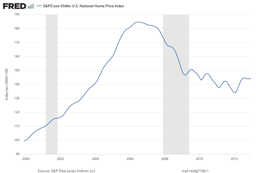
It is a widely held belief that the problems in financial markets and the U.S. macroeconomy that triggered the Great Recession of 2008-09 had their origins in the decline in the U.S. housing market. There appears to be considerable evidence to support this claim. By many estimates, prior to the bubble bursting, the U.S. housing market inflated to $8 trillion beyond historic norms. As unstable as the housing boom was, rising house prices did increase household wealth and contributed to the growth of aggregate demand. After the housing market collapsed, as residential real estate prices fell, household wealth was extinguished which contributed to declining aggregate demand. More significantly, the decline in housing prices was the engine behind the collapse of financial markets.
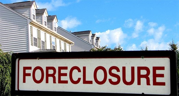
As residential housing prices declined, mortgage debt became an unreliable source of income for financial market institutions responsible for issuing mortgage debt. For many borrowers, as house prices fell the price of their home declined below the original purchase price and this caused many borrowers to be pushed into default. Defaults, of course, lead to foreclosures which further suppressed housing prices and, subsequently, exacerbated the cycle of economic contraction and decline. For financial institutions, however, the story did not end with foreclosures.
In terms of the overall financial market, as residential housing prices declined, the flow of income generated by mortgage debt became unreliable because the assets derived (“derivatives”) from the mortgages issued on those homes became unstable. The mortgage backed securities (MBS), as well as derivatives of those securities, became less valuable. If a financial institution counted MBSs as a part of their balance sheet, then as MBSs fell in value, the financial institution’s liabilities began to rise relative to the now falling MBS asset prices. The result was that MBSs that were previously useful as collateral, became a noose around the neck of financial institutions. Without collateral it became difficult to secure loans. In this case, financial institutions were both unwilling to lend and incapable of securing loans. The result was a freezing of credit markets and a financial collapse. Strikingly, what this meant was that as housing prices fell, lenders had increasing difficulty in issuing new loans, which meant that even good borrowers had difficulty securing loans. In the absence of access to credit, regardless of how low housing prices fell, consumers were not able to borrow adequate funds to purchase now less expensive homes. Naturally, the absence of demand caused housing prices to fall further and the process continued.
Clearly as residential housing prices declined and the financial turmoil continued in financial markets, it would seem that the housing market could have benefited from price stickiness. While the $700 billion Troubled Asset Relief Program (TARP) financial market bailout eased some of the pressure on credit markets, without housing price stabilization, the financial markets as well as the macroeconomy in general continued to experience decline. Had the heterodox interpretation of price adjustments been applied, the government would have tailored its policies toward remedying the destabilizing aspects of housing market deflation and mortgage derivative deflation. So long as housing prices continued to decline, average Americans continued to lose their homes to foreclosure and the debt-deflation spiral continued.
Housing Market Deflation
The 2008-2009 Great Recession hit the U.S. economy hard, representing the worst recession since the Great Depression According to the Bureau of Labor Statistics (BLS), the number of unemployed Americans rose from 6.8 million in May 2007 to 15.4 million in October 2009. During that time, the U.S. Census Bureau estimated that approximately 170,000 small businesses closed. Mass layoffs peaked in February 2009 when employers gave 326,392 workers notice. U.S. productivity and output fell as well. Job losses, declining home values, declining incomes, and uncertainty about the future caused consumption expenditures to decrease. According to the BLS, household spending dropped by 7.8%.
Home foreclosures and the meltdown in U.S. financial markets generated calls for immediate action by Congress, the President, and the Federal Reserve Bank. While many prominent heterodox economists called for a large multi-trillion dollar government spending package, prominent New Keynesian economists within the Obama Administration such as Christina Romer (the Chair of the Council of Economic Advisers) and Larry Summers (National Economic Council) proposed a $500-$800 billion package. For example, the government implemented programs such as the American Restoration and Recovery Act to help millions of people by providing tax credits for homebuyers, paying “cash for clunkers,” and extending unemployment benefits. From cutting back on spending, filing for unemployment, and losing homes, millions of people were affected by the recession. What caused this recession and what prevented the economy from spiraling further into another depression? Some Policymakers evaluated the lessons learned from the 1930s Great Depression considered Keynes’ models to analyze the causes and find solutions to the country’s economic woes. Leading into the Great Recession, housing prices hit their peak in 2006, the average price of housing in the United States then fell significantly.
For many economists, as well as some pundits, prognosticators, and even members of the United States congress the decline in the price of housing was to be applauded. Consider, this statement by Libertarian leaning Republican congressman Ron Paul,
When builders realize they have overbuilt and have too many houses to sell, too many apartments to rent, or too much commercial real estate to lease, they seek to recoup as much of their money as possible, even if it means lowering prices drastically. This lowering of prices brings the economy back into balance, equalizing supply and demand.
So, the orthodox economic argument went during the Great Recession, the fastest way to a housing market recovery, as well as a macroeconomic recovery, is for prices to fall until consumers can once again afford to make purchases. This thinking, however, relies on faith in a free market ideal that, when put into practice, has the potential to continue to destabilize the economy. In his ever prescient classic, The General Theory, John Maynard Keynes’ theoretical framework warned about the macroeconomic dangers associated with deflation.
Ultimately, in the immediate aftermath of the economic trough associated with the Great Recession, the U.S. economy resumed growing, but did so at arguably slowest rate coming out of a downturn as any contraction in the Post-Great Depression era.
Keynes and the Aggregate Demand/Aggregate Supply Model
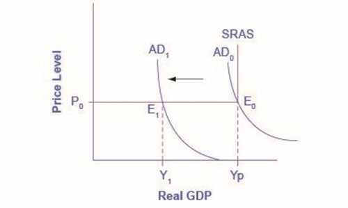
Many orthodox economists believe that, once issues like sticky wages and prices are recognized, the simplified AD/AS model that we saw in Chapter “The Aggregate Demand-Aggregate Supply Model” is fully consistent with Keynes’s original model. Figure 2, below, is the AD/AS diagram which illustrates two basic Keynesian assumptions—the importance of aggregate demand in causing recession and that if an economic contraction occurs it will continue until the economy stabilizes with sticky wages and prices at less a than full employment outcome. stickiness of wages and prices. Note that in an economic trough, because of the stickiness of wages and prices, flattens the aggregate supply curve. is flatter than either supply curve (labor or specific good). In fact, if wages and prices were so sticky that they did not fall at all, the aggregate supply curve would be completely flat below potential GDP, as Figure 2 shows. This outcome is an important example of a macroeconomic externality, the fallacy of composition where what happens at the macro level is different from and inferior to what happens at the micro level. For example, a firm should respond to a decrease in demand for its product by cutting its price to increase sales. However, if all firms experience a decrease in demand for their products, sticky prices in the aggregate prevent aggregate demand from rebounding (which we would show as a movement along the AD curve in response to a lower price level).
The original Keynesian argument notes that an economy can settle at multiple points of equilibria. It is possible for the equilibrium of this economy to occur where the aggregate demand function (AD0) intersects with AS. Since this intersection occurs at potential GDP (Yp), with the economy is operating at full employment. At the same time, once an economy has contracted into a depressionary state, when aggregate demand shifts to the left, all the equilibrating adjustment occurs by virtue of a reduction in through decreased real GDP. Because this illustration represents an economy that has contracted to a recessionary state and There is no decrease in the price level. Since the equilibrium occurs at Y1, the economy experiences substantial unemployment.
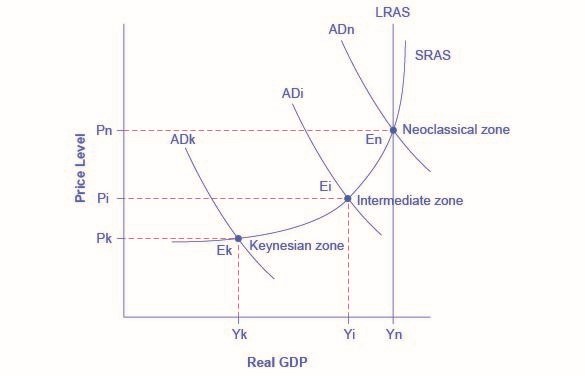
More recent research, though, has indicated that in the real world, an aggregate supply curve is more curved than the right angle depicted in the figure above. Because the economy does not always operate in a depressed or recessed state, one way to try to provide a more Rather, the real-world reflection of the AS curve is that very flat at levels of output far below potential (“the Keynesian zone”), very steep at levels of output above potential (“the neoclassical zone”) and curved, as the economy transitions from expansions to contractions or vice versa, in between (“the intermediate zone”). Figure 3 illustrates this. The typical aggregate supply curve leads to the concept of the Phillips curve.
occurs when what happens at the macro level is different from and inferior to what happens at the micro level; an example would be where upward sloping supply curves for firms become a flat aggregate supply curve, illustrating that the price level cannot fall to stimulate aggregate demand
