
32.4 – Prices from Pricing
Learning Objectives
By the end of this section, you will be able to:
- Identify the basic pricing methods of unit cost pricing and target rate of return pricing
- Calculate prices according to these methods
- Discuss the implications of planning, costing, and pricing for the existence of a supply curve
In the previous section, you learned about how costs are recognized in the accounting of a modern business enterprise. This process depends on the accounting practices and policies of the company, as well as the regulations, historical norms and laws, and so on under which the company operates. Costs, indeed, are hardly just given mathematical functions derived from market prices and production functions. In this section, we’ll see that prices are, similarly, created by the decisions being made within these businesses operating as going concerns.
Prices from Pricing
Similar to costing, pricing refers to procedures businesses use to determine, beforehand, the price at which they will sell their product once production is up and running and sales can be made. While modern pricing procedures can be complex and will vary widely across different businesses and industries, we’ll look at two basic methods here: unit cost pricing and target rate of return pricing. Both are instances of markup (or cost-plus) pricing: setting the price of a business enterprise’s product by adding some amount over and above the average cost of production.
Unit cost pricing is the simpler of the two methods. It can be written as
[latex]P = (ATC)(1 + r)[/latex]
Where:
P is the price at which the business plans to sell its product
ATC is the average total (or per-unit) cost determined in the costing process
r is the predetermined markup
Target rate of return pricing is similar, but a bit more complicated. Here the price is being set, not to achieve a particular percentage profit above costs, but to earn a desired return on the money invested into the business. The formula can be written as
[latex]P = ATC + \frac{(ROI) \times (IC)}{Q}[/latex]
Where:
ROI is desired return on invested capital
IC is invested capital–that is, money invested into producing the product
Q is the expected quantity of output sold
Calculating Prices
To illustrate both pricing methods, consider a business that invests $10 million into a plant designed to manufacture inexpensive steak knives. It expects that over some relevant period it will be able to produce and sell 2 million knives, and, at that level of production, its per-unit costs will be $1.80 per knife. This figure would be calculated by adding up the estimated costs of labor, materials, overhead, depreciation on fixed capital, and so on, then dividing by the 2 million units of expected sales. The calculated prices using our two pricing procedures are given below (assuming that in the first case the desired markup is 10% (or 0.1), and in the second the desired return on invested capital is also 10%).
Unit cost price: [latex]P = (\$1.80)(1 + 0.1) = \$1.98[/latex]
Target rate of return price: [latex]P = \$1.80 + \frac{(0.1) \times (\$10,000,000)}{2,000,000} = \$2.30[/latex]
Notice that, even though the markup and desired return on invested capital are both 0.1 (10%), the resulting markups and hence the prices are not the same. This is because, although both procedures are essentially marking the price up over costs, the way the markup is determined is different.
Pricing and Profits
Figure 1, below, depicts the essential features of our heterodox model of costing and pricing. The cost curves are the same as you saw earlier in the chapter, with marginal cost constant (which means it’s the same as average variable cost), and average fixed and total costs simply declining as output increases. The dashed vertical line, QP, shows the planned level of output and sales of the business at 600 units, which corresponds roughly to $52 cost per unit. The price, P, is set at $75, representing a 45% markup over unit cost.
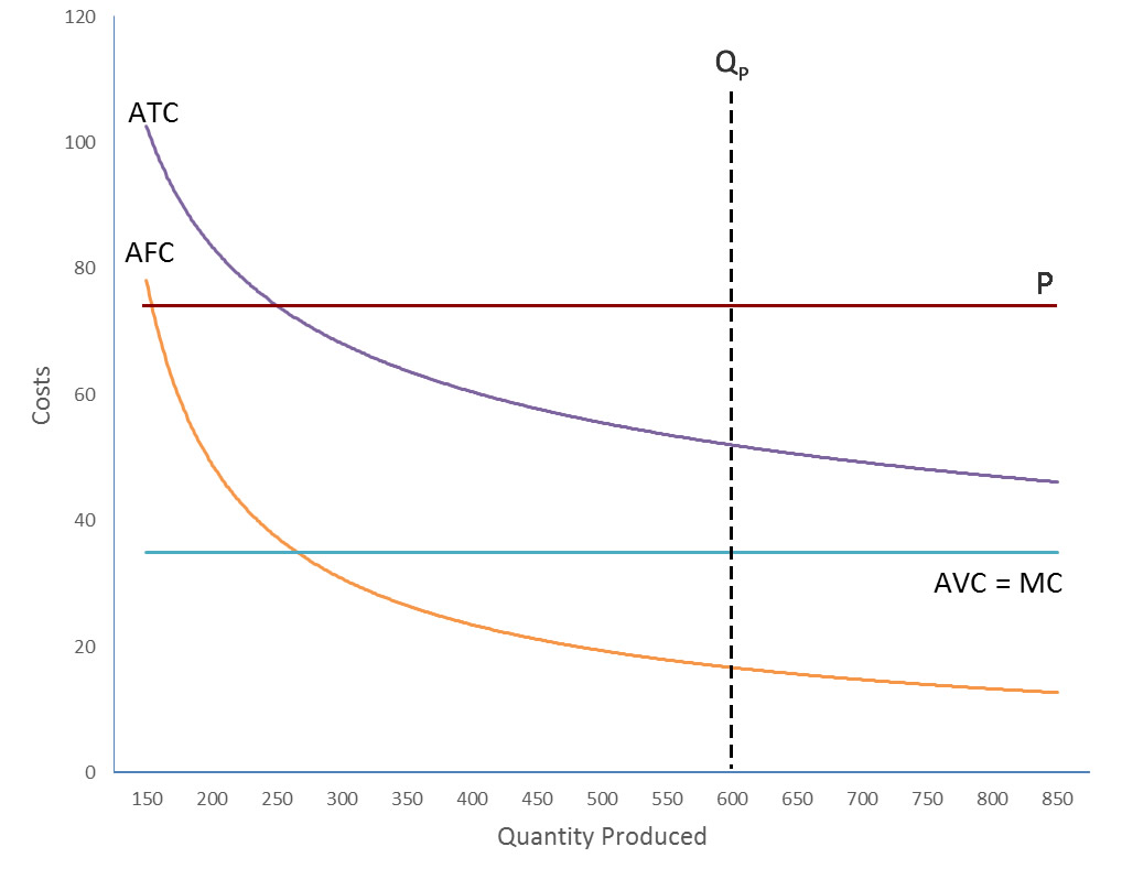
Note that in Figure 1 the price curve is represented as a horizontal line at $75. Graphically, our heterodox model shows a constant price just like the one depicted in chapter “Perfect Competition”, however the interpretation here is completely different. In the orthodox model of perfect competition, firms are ‘price takers’, meaning the market–that is, the interaction of supply and demand–determines the price, and the firm simply decides which quantity to sell at that price so as to maximize profits. In contrast, the heterodox model depicted in Figure 1 shows a constant price determined not by the market but by the business enterprise itself (according to some particular markup process). The business then sets that price, ‘announcing’ it, so to speak, to the market and selling as much as people are willing to buy. That price is not—indeed, cannot be—profit maximizing, and the quantity can only be guessed at ahead of actually coming to the market.
In short, whereas the orthodox model has the market determining the price and the firm determining the quantity it wishes to produce and sell, the heterodox model has the firm determining its price and the market determining the quantity the firm will ultimately produce and sell.
One consequence of the heterodox model is that profit is, in a sense, both created by the business and at the same time fundamentally uncertain. Profit is created when the business decides how much to mark up its costs to determine its price; but it ultimately remains an uncertain thing because the business never knows for sure if it is actually going to hit its planned sales target or budgeted costs.
Prices as Part of Planning
It is worth reflecting on the significance of these insights into cost accounting and markup pricing, as they represent important general concepts in heterodox economics which are usually neglected in standard orthodox theory. First, they suggest that business enterprises are making decisions before anything is even produced, let alone brought to market. In particular, pricing practices (as well as the quantity of output and sales, and the corresponding cost estimates on which pricing is based) are a component of the planning process which takes place within the business enterprise. While not entirely neglectful of demand and market conditions, this process is taking place on the supply side, by the businesses, and the market transactions for which the planning process is being done are only hypothetical future events during the planning process itself. And contrary to the axiom that firms cannot recover fixed costs in the short run and therefore should ignore them in making short run decisions, it is this long run planning process driving short run behavior that is most important for understanding what determines prices.
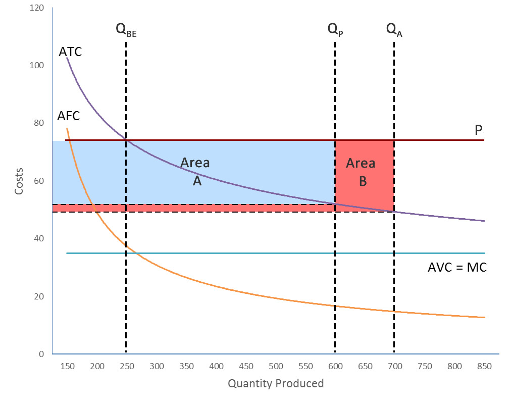
Second, to acknowledge costing and pricing as it actually occurs is to acknowledge that the future is fundamentally unknowable. While standard (orthodox) models assume that firms know their production costs and, typically, also the amount they can sell and the resulting revenues they can expect to take in, actual firms face uncertainty in how their plans will work out. A particular implication of this reality: since firms set prices based on estimated average total cost at an expected level of output, a change in the actual quantity of production/sales is unlikely to affect the predetermined price. This suggests that price and quantity supplied are determined completely separately, which in turn means that there is no such thing as a supply curve.
The Illusory Supply Curve
Recall from the basics of the neoclassical market model that a supply schedule (and its corresponding supply curve) shows how much a firm (or firms) would be willing to supply at various market prices. That is, supply simply refers to the functional relationship between quantity supplied and the market price, with the market price determining the quantity supplied. If, however, the two are determined separately then there’s no way around the implication that quantity supplied is not functionally related to the market price–that is, there is no supply curve.
The astute reader may have already realized the impossibility of supply curves under certain conditions from the failed hypotheses discussed earlier in this chapter. Referring back to chapter “Perfect Competition,” specifically the section titled “Marginal Cost and the Firm’s Supply Curve,” you’ll recall that a firm’s marginal cost curve (above minimum average variable cost) is its supply curve. (This is because quantity supplied is determined where MC = MR and, under perfectly competitive conditions, MR = P. Hence, quantity supplied is determined by P = MC.) Now, as was shown earlier in this chapter with the test of hypothesis 2, firms simply couldn’t determine their quantity supplied this way—at least not under competitive conditions and having the empirically typical average total cost curves. This, of course, means that the neoclassical theory of supply must be rejected for these cases.
This doesn’t mean that the basic ideas of supply–higher prices leading to higher output and vice versa, for instance–are completely absent in the real world. Some industries–particularly, those related to mining and agriculture–sometimes do see diminishing returns. One could argue that, in these relatively small parts of modern economies, upward-sloping supply curves may be found. However, as our examination of the cost structures of actual firms suggested earlier in this chapter, this relegates what is considered the normal case in orthodox economics to a special—and pretty rare—case.
Third and finally, a review of the evidence and history of actual businesses reveals an anachronism within the orthodox theory of the firm. As you learned in chapter “Perfect Competition,” the firm chooses the most profitable line of business (and appropriate production technique) in the long run, and the profit maximizing quantity to produce in the short run. If in the short run the firm is making a loss, it will choose to shut down if its fixed cost losses would be lower than the losses on continuing production. In an abstract but important way the business enterprise this theory is describing is a terminal venture. Yet, beyond the halls and offices of economics departments at least, firms are generally seen as going concerns. This is reflected, for instance, in the accounting practices discussed above, as well as in the relationships firms maintain with customers. Blinder and colleagues (1998, pp. 96-7) found that 85% of all sales in the economy are made to regular customers whom the business expects to sell to in the future. In manufacturing and wholesale trades that number is over 90%.
As will be explored in more depth in the next chapter, the idea that businesses are organized and run as going concerns is a significant theoretical innovation over the standard orthodox theory of the firm. For now, we only need to consider what it means for prices. The importance of the price mechanism—the ‘invisible hand of the market’—in the overarching story of orthodox economics cannot be overstated. It is the process by which self-interested people (consumers, workers, entrepreneurs, landlords, and all the rest) are brought together in exchange for all of their mutual benefit. It is the mechanism that allows economists to believe in a (potentially) optimal equilibrium state–in an individual market, and in a capitalist economy as a whole.
In contrast, what is being argued in this section is that prices—at least those prices not actually determined through an auction—are set by businesses themselves as part of their planning process. The reader may have noticed that in the markup pricing introduced above a glaring question was ignored: namely, what determines the markup? A succinct, if incomplete answer can now be given: if the firm is to be a going concern, the markup, as well as the procedures that determine costs, will reflect the needs of the firm to continue to do business into the foreseeable future. For most firms there will also be plans to grow. Hence, from this view, prices are not exchange-based, market clearing values at all. They are, rather, reproduction prices–allowing the firm to reproduce itself through time–and, typically, also growth prices–ensuring the firm brings in the earnings necessary to expand. To use a now-familiar term, the vast majority of the prices we see in actual capitalist economies today might best be called going concern prices.
Making the Numbers
One of the important takeaways from this and the previous section is that costs and prices are not mechanically determined by technology and consumer preferences as the supply-and-demand model would suggest. Rather, costs are created by accounting conventions and managerial expectations within businesses, and costs are often shifted onto others where possible. Prices, then, are typically determined through a markup process on those costs, and the markup is similarly a creation of management planning. The emphasis in this heterodox perspective is on what managers do, and you’ll learn more about this perspective in the next chapter. But, before moving on, it’s worth considering the role of the owners of these businesses, who for most large corporations are not the same people as the management. The owners of corporations are their shareholders, and those shares are often held not by an individual but by a mutual fund, hedge fund, or private equity firm.
For most of the twentieth century, these shareholders were relatively passive. Part of a company’s profit would be handed over to the shareholder in the form of dividends, and if a shareholder didn’t like the way the company was being run, they would simply sell the shares. In the 1980s, however, hostile takeovers became relatively common. These occur when shareholders, usually organized as a private equity firm, buy enough of the company’s outstanding shares to allow them to replace the top management (the takeover of the company is hostile in the sense that current management opposes it). Because of this threat from organized shareholders, corporate managers have, since the 1980s, been more concerned with ‘maximizing shareholder value’, meaning the markup—or at least windfall profits arising from lower costs, higher sales, or tax cuts—have been channeled increasingly to financial firms.
You can learn more about this historical trend in chapter “The Surplus and the Price Level”. For now it is worth considering again what determines costs and prices. For most of what is produced in a modern capitalist economy, both costs and prices are not given, but are created by managers, accountants, and the like. And while it’s still true that the markup over costs mainly functions to finance a business’ investments, and thereby allowing it to maintain itself as a going concern, it is also true today that financial firms have a strong claim on those same funds.
Glossary
- Going concern prices
- a concept of prices as being determined by the particular needs of the businesses setting their prices to allow themselves to survive and grow
- Markup pricing
- setting the price of a business enterprise’s product by adding some dollar amount over and above average costs of production. Full cost pricing and target rate of return pricing are two examples
- Pricing
- procedures businesses use to determine, beforehand, the price at which they will sell their product once production is up and running and sales can be made
procedures businesses use to determine, beforehand, the price at which they will sell their product once production is up and running and sales can be made
setting the price of a business enterprise’s product by adding some dollar amount over and above average costs of production. Full cost pricing and target rate of return pricing are two examples
a concept of prices as being determined by the particular needs of the businesses setting their prices to allow themselves to survive and grow
