
13.4 – The Corn Model: Production with a Surplus
Learning Objectives
By the end of this section, you will be able to:
- Analyze a corn model with a surplus and equal profit rate across sectors
- Explain how the corn model fits into the broader body of heterodox economic theory
In the previous section, we looked at the math of our corn model involving an economy that produces just enough output to have the inputs it will need in the next year to continue producing. But this only scratches the surface of what we can show with this model. Actual economies don’t simply produce just enough to keep going–that would be a very precarious situation, indeed. Instead, they produce a surplus. Considering first, as we did in the previous section, how an economy can undergo a process of simple reproduction helps to illustrate the concepts of viability and the Going Economy. A much more interesting and practical consideration is the case where an economy accumulates output as surplus, and does so period after period.
Recall that earlier in the chapter we stated that the Surplus Approach is defined by its emphasis on both the quantity and the quality of the surplus. Before we proceed with some arithmetic and charts to illustrate expanded reproduction in the case of surplus, let us consider some interesting qualitative aspects of an economy’s surplus.
First, the surplus – that is the output produced over and above that which is required to supply the various industries with the requisite materials and resources for reproduction – does not spring forth as ‘mana from heaven.’ Rather, it is the result of past investment decisions on the part of either private or public actors. These investments created new plant and equipment capable of transforming labor and other resources into other goods, and in the process changed the structure of interdependence for the economy as a whole. Specifically, the type of goods that result from that past investment and ultimately accrue as measured surplus output reflect the priorities for the economy attendant to that investment choice. One can envision a boundless array of potential investment choices a society can make. However, over a given time horizon, there is a finite and discrete set of possibilities for the way in which the surplus can be arranged, and those outcomes are ‘locked in’ by investments of a prior day. So in this sense, while we can measure quantitative changes in the value of the output of the surplus, we are only getting half the picture if that’s all we focus on. It’s important also to think about what the surplus provides for us in terms of resources, how the economy as a whole is arranged to produce them, and for whom they are produced.
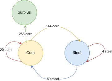
Returning to our hypothetical economy, producing only corn and steel, suppose the following. The corn sector uses 20 tons of corn and 80 tons of steel to produce 420 tons of corn, while the steel sector uses 144 tons of corn and 4 tons of steel to produce 84 tons of steel. We can write this as:
[latex]20 \text{ corn} + 80 \text{ steel} → 420 \text{ corn} \\ 144 \text{ corn} + 4 \text{ steel} → 84 \text{ steel}[/latex]
First, we can check to see if this economy is viable the same way we did in the previous section. We’ll start with steel. The corn sector uses 80 tons of steel while the steel sector uses 4 tons, so if the economy is going to be able to continue producing next year, the steel sector needs to make at least 80 + 4 = 84 tons of steel. And we see that it does just that, so the economy is viable in terms of steel.
Now for corn. The corn sector uses 20 tons of corn while the steel sector uses 144 tons, meaning the corn sector needs to be producing at least 20 + 144 = 164 tons of corn. We can see that it does indeed meet that threshold, so the economy is technically viable in terms of both its products. However, we can also see that the corn sector produces well above the 164 tons needed to continue production–specifically, it’s producing 420 – 164 = 256 tons of corn more than is necessary. This is the surplus. Figure 1 depicts the interaction of our two sectors now, including the production of the surplus.
The next question, then, is what prices–corn relative to steel or vice versa–will allow each sector to afford the inputs it needs. The math gets a bit trickier here than the last section, so we’ll just look at how we would go about answering this question, and save the actual solving of the problem for later in the chapter.
It turns out that once we have a surplus to deal with, determining the relative prices of corn and steel can’t be done without assuming something about how the surplus will be distributed. Since we have in mind a capitalist economy, it makes sense to think of the surplus as going to profit. And, as one final assumption, we’ll say that the rate of profit is equal between the two sectors.
Here profits are the value of the output each sector sells (that is, its revenues) over and above the cost of the inputs used. And the rate of profit is given by the profits divided by the cost, expressed as a percentage. (For example, if a sector had $110 in revenues and $100 in costs, then its profits would be [latex]$110 - $10 = $10[/latex] and its rate of profits would be [latex]\frac{$10}{$100} = 0.1 = 10\%[/latex].) We’re assuming, then, that the percentage is the same for both sectors.
Let’s find the rate of profits for the corn sector. First we want to know the profits. This is going to come from the revenues of the 420 tons of corn sold, but bearing in mind that 20 tons of corn were used up in production and that 80 tons of steel were purchased, both of which count as costs to corn sector production. Hence, our profits–not yet in dollar terms, but rather the quantities of the actual products–are:
[latex]\text{Profits}_\text{corn} = \text{Revenues} - \text{Costs} = 420 \text{ corn} - (20 \text{ corn} + 80 \text{ steel})[/latex]
To find the rate of profit, then, we simply divide the profits by the costs:
[latex]\text{Rate of profit}_\text{corn} = \frac{\text{profits}}{\text{costs}} = \frac{420 \text{ corn} - (20 \text{ corn} + 80 \text{ steel})}{20 \text{ corn} + 80 \text{ steel}}[/latex]
Now, onto the steel sector. This will actually be simpler than the corn sector, since the steel sector doesn’t produce a surplus–that is, it only makes just enough steel to cover the inputs of both sectors–although, as we’ll see, it does get a share of the corn surplus. In this case, we can think of the steel sector’s revenues as simply the value of the steel it sold to the corn sector (80 tons of steel), and its costs as the value of the corn it purchased from that sector (144 tons of corn). Hence, steel sector profits are:
[latex]\text{Profits}_\text{steel} = \text{Revenues} - \text{Costs} = 80 \text{ steel} - 144 \text{ corn}[/latex]
The rate of profit is found just as we did with the corn sector:
[latex]\text{Rate of profit}_\text{steel} = \frac{\text{profits}}{\text{costs}} = \frac{80 \text{ steel} - 144 \text{ corn}}{144 \text{ corn} + 4 \text{ steel}}[/latex]
Having set up the rates of profits for each sector, we now only need to refer to our assumption about how they relate. Specifically, we’re going to assume that the rate of profits is equal between the two sectors, which we can write as:
[latex]\text{Rate of profit}_\text{steel} = \text{Rate of profit}_\text{corn}[/latex]
[latex]\frac{420 \text{ corn} - (20 \text{ corn} + 80 \text{ steel})}{20 \text{ corn} + 80 \text{ steel}} = \frac{80 \text{ steel} - 144 \text{ corn}}{144 \text{ corn} + 4 \text{ steel}}[/latex]
As noted above, we won’t solve this equation here as the math is fairly involved (but you can see a similar example and its complete solution at the end of the chapter). It is enough here to say that the above equation, once solved, suggests that 1 ton of steel is worth 3 tons of corn–which means that, whatever the price of corn is, steel should be priced at 3 times that amount.
Let’s suppose, then, that corn costs $10 per ton, suggesting that steel costs $30 per ton. We can look back to our previous equations for profits and the rate of profit for each sector and see what those come out to be. To do this, simply multiply each of the numbers that’s followed by ‘corn’ by 10 and each number followed by ‘steel’ by 30 to get their dollar values.
For the corn sector:
[latex]\text{Profit}_\text{corn} = $4,200 - $200 - $2,400 = $1,600[/latex]
[latex]\text{Rate of profit}_\text{corn} = \frac{$1,600}{$200 + $2,400} = \frac{$1,600}{$2,600} = 0.6154 = 61.54\%[/latex]
And for the steel sector:
[latex]\text{Profit}_\text{steel} = $2,400 - $1,440 = $960[/latex]
[latex]\text{Rate of profit}_\text{steel} = \frac{$960}{$1,440 + $120} = \frac{$960}{$1,560} = 0.6154 = 61.54\%[/latex]
Notice that, even though only one sector produces the surplus (corn), both sectors share in the surplus as relative prices are set so as to ensure an equal rate of profits. But note, further, that although both sectors enjoy the same rate of profits (which we had assumed at the outset), they don’t earn the same profits in dollar terms. This is because the rate of profit is a percentage over outlays–that is, the costs of inputs used in the sector–so the actual profits are different because the sectors’ outlays are different. So, for those in the corn business, profits come out collectively to $1,600, whereas steel companies on the whole only earned profits of $960. But notice that total outlays in the corn sector came out to 200 + 2,400 = $2,600, while steel outlays were only 1,440 + 120 = $1,560. Hence, while the steel companies brought in less in total profits than the corn companies, they still made the same return per dollar invested.
So there you have it: provided that we are able to say something about the distribution of the surplus, it is possible to derive the relative prices of the various products an economy produces simply by reference to the quantities each sector uses as inputs and how much each sector produces as an output. We’ve demonstrated this with a hypothetical economy that produces only two outputs, each of which is necessary in the production of both itself and the other product. But the logic we’ve used in this section could be applied to any number of products, and indeed could include luxury-type products that are not necessary to the production of any other product.
We could also expand this model to include other sectors that lie at critical input-output junctures, like labor and ecological services. In fact, for the sake of simplicity labor in the model we’ve been looking at is collapsed into the cost of production for each of the two sectors we’ve considered, but a more complex (and realistic) version of the model would not do this. Instead, we would recognize that there are distinct labor and production pairings that are particular to each industry, and which are subject to distributional arrangements that allow for wages to be paid from the surplus as well as profits. A similar story can be told via surplus approach models for the ecology, with direct and relevant connections between viability and sustainability! What’s interesting about this approach is that in either case, there is an explicit recognition that power is central to the analysis and not something that simply disappears in the model or is assumed away.
How the Corn Model fits into heterodox economics more broadly
The model we’ve been discussing in this chapter is useful for explaining (relative) prices throughout the entire economy without needing to make reference to demand and supply curves, either at the individual market level or in the aggregate. That is to say our Corn Model doesn’t need the standard tools of orthodox economics to do its job. But you might ask, how does this fit in with the rest of heterodox economics, micro and macro? Two important ways are worth noting. First, at the macroeconomic level, you have learned (or will learn) in chapter “A Heterodox Macroeconomic Perspective” that heterodox economists believe that capitalist economies adjust to imbalances between total spending and total output and employment, not through price changes, but rather through changes in output and employment. Our corn model here lines up perfectly with this view, since it gives an explanation for prices that doesn’t refer to aggregate demand or aggregate supply. Indeed, we can go further in applying the Corn Model to the real world and say that when prices are not exactly in line with the reproduction prices of our model, industries are likely to compensate through inventory and capacity utilization adjustments rather than price adjustments. That is to say, the perpetual change and disequilibrium of actual capitalist economies involve primarily quantity rather than price adjustments–a key argument that distinguishes heterodox from orthodox economics.
Second, at the microeconomic level, chapter “Costing and Pricing in Going Concerns”, discusses pricing for individual businesses. In essence, that chapter explains heterodox theory in terms of businesses marking up their prices over estimated average costs. This profit markup, the difference between costs per unit and the price, serves the purpose of funding whatever the business needs to do to remain a going concern. The similarity between that approach, at the microeconomic level, and this chapter’s Corn Model, at the macroeconomic level, should be fairly obvious. Both are parts of the general body of heterodox economic theory treating prices as a process of covering the costs of production with an addition for profits. Likewise, both look at the issues in question in terms of reproducibility or going concerns.
