
39.2 – Labor markets
Learning Objectives
By the end of this section, you will be able to:
- Describe the demand for labor in perfectly competitive output markets
- Describe the demand for labor in imperfectly competitive output markets
- Identify what determines the going market rate
What is a labor market?
The labor market is the term that economists use for all the different markets for labor. There is no single labor market. Rather, there is a different market for every different type of labor. Labor differs by type of work (e.g. retail sales vs. scientist), skill level (entry level or more experienced), and location (the market for administrative assistants is probably more local or regional than the market for university presidents). While each labor market is different, they all tend to operate in similar ways. For example, when wages go up in one labor market, they tend to go up in others too. When economists talk about the labor market, they are describing these similarities.
The labor market, like all markets in the orthodox approach, has a demand and a supply. Why do firms demand labor? Why is an employer willing to pay you for your labor? It’s not because the employer likes you or is socially conscious. Rather, it’s because your labor is worth something to the employer–your work brings in revenues to the firm. How much is an employer willing to pay? That depends on the skills and experience you bring to the firm.
If a firm wants to maximize profits, it will never pay more (in terms of wages and benefits) for a worker than the value of his or her marginal productivity to the firm. We call this the first rule of labor markets.
Suppose a worker can produce two widgets per hour and the firm can sell each widget for $4 each. Then the worker is generating $8 per hour in revenues to the firm, and a profit-maximizing employer will pay the worker up to, but no more than, $8 per hour, because that is what the worker is worth to the firm.
Recall the definition of marginal product. Marginal product (of labor) is the additional output a firm can produce by adding one more worker to the production process. In this chapter, we assume that workers are homogeneous—they have the same background, experience and skills and they put in the same amount of effort. It follows, then, that marginal product depends on the capital and technology with which workers have to work. A typist can type more pages per hour with an electric typewriter than a manual typewriter, and he or she can type even more pages per hour with a personal computer and word processing software. A ditch digger can dig more cubic feet of dirt in an hour with a backhoe than with a shovel.
In the short run, however, we know that at least one input to production is fixed and at least one is variable. It makes sense for us here to say that the capital is fixed and the number of workers is variable. With this in mind, we can look at the additional output each additional worker produces, understanding that the capital (computers, shovels, grills in a kitchen, or what have you) doesn’t change. This should give us a marginal product of labor that looks something like the table and graph below.
| # Workers (L) | 1 | 2 | 3 | 4 |
| MPL | 4 | 3 | 2 | 1 |
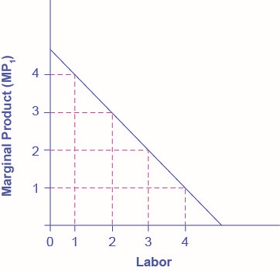
Figure 1 Marginal Product of Labor Because of fixed capital, the marginal product of labor declines as the employer hires additional workers.
Notice that each additional worker adds a smaller amount of additional output than the previous worker–there are diminishing returns to hiring more workers. This is simply the result of the fixed capital assumption: more workers without more capital to work with will make the workers themselves less productive as, for instance, they have to take turns using the shovels or the kitchen gets crowded with cooks.
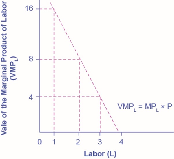
Now, the more important question for the employer is: what’s the actual monetary value of each additional worker’s marginal product? If we assume that the employer sells its output in a perfectly competitive market, the value of each worker’s output will be the market price of the product. Thus,
Demand for Labor = MPL x P = Value of the Marginal Product of Labor
We show this in Table 2, which is an expanded version of Table 1.
| # Workers (L) | 1 | 2 | 3 | 4 |
| MPL | 4 | 3 | 2 | 1 |
| Price of Output | $4 | $4 | $4 | $4 |
| VMPL | $16 | $12 | $8 | $4 |
Note that the value of each additional worker is less than the ones who came before.
Demand for Labor in Perfectly Competitive Output Markets
The question for any firm is how much labor to hire.
We can define a Perfectly Competitive Labor Market as one where firms can hire all the labor they wish at the going market wage. Think about secretaries in a large city. Employers who need secretaries can probably hire as many as they need if they pay the going wage rate.
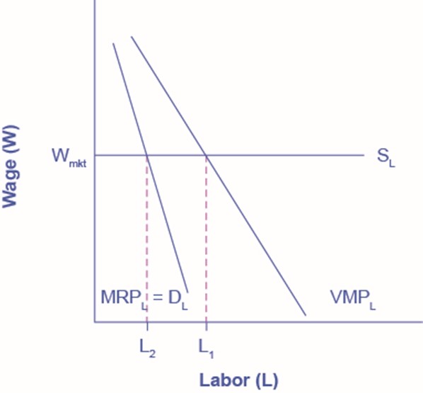
Graphically, this means that firms face a horizontal supply curve for labor, as Figure 3, below, shows.
Given the market wage, profit maximizing firms hire workers up to the point where: Wmkt = VMPL.
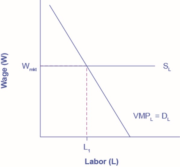
Here, the quantity in question isn’t the quantity to produce, but rather the quantity of workers to hire (L). The marginal cost is simply the market wage (Wmkt), which is constant. The marginal revenue is the value (that is, revenues) of the marginal product each additional worker produces (VMPL). Hence, the the intersection of Wmkt and VMPL in our labor market here is the profit maximizing point for hiring labor, just as the intersection of MC and MR is the profit maximizing point for producing a product in chapter “Perfect Competition“.
Derived Demand
Economists describe the demand for inputs like labor as a derived demand. Since the demand for labor is MPL*P, it is dependent on the demand for the product the firm is producing. This is implied by the V term (for monetary value) in VMPL, which is the demand for labor. An increase in demand for the firm’s product drives up the product’s price, which increases the firm’s demand for labor. Thus, we derive the demand for labor from the demand for the firm’s output.
Demand for Labor in Imperfectly Competitive Output Markets
If the employer does not sell its output in a perfectly competitive industry, they face a downward sloping demand curve for output, which means that in order to sell additional output the firm must lower its price. This is true if the firm is a monopoly, but it’s also true if the firm is an oligopoly or monopolistically competitive. In this situation, the value of a worker’s marginal product is the marginal revenue, not the price. Thus, the demand for labor is the marginal product times the marginal revenue.
The Demand for Labor = MPL x MR = Marginal Revenue Product
| # Workers (L) | 1 | 2 | 3 | 4 |
| MPL | 4 | 3 | 2 | 1 |
| Marginal Revenue | $4 | $3 | $2 | $1 |
| MRPL | $16 | $9 | $4 | $1 |
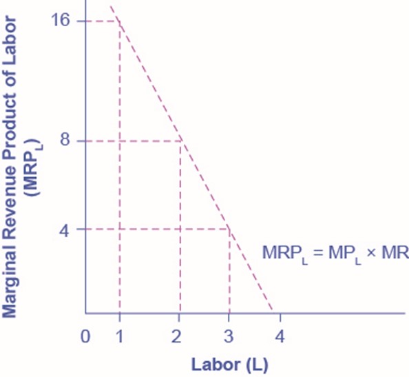
Everything else remains the same as we described above in the discussion of the labor demand in perfectly competitive labor markets. Given the market wage, profit-maximizing firms will hire workers up to the point where the market wage equals the marginal revenue product, as Figure 5 shows.
What Determines the Going Market Wage Rate?
In the chapter “Labor and Financial Markets“, we learned that the labor market has demand and supply curves like other markets in orthodox economic theory. The demand for labor curve is a downward sloping function of the wage rate. The market demand for labor is the horizontal sum of all firms’ demands for labor. The supply of labor is an upward sloping function of the wage rate. This is because if wages for a particular type of labor increase in a particular labor market, people with appropriate skills may change jobs, and vacancies will attract people from outside the geographic area. The market supply for labor is the horizontal summation of all individuals’ supplies of labor.
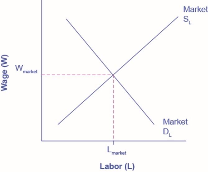
Like all equilibrium prices, the market wage rate is determined through the interaction of supply and demand in the labor market. Thus, we can see in Figure 7 for competitive markets the wage rate (or price) and number of workers hired (quantity).
The FRED database has a great deal of data on labor markets, starting at the wage rate and number of workers hired.
The Bureau of Labor Statistics publishes The Current Population Survey, which is a monthly survey of households, which provides data on labor supply, including numerous measures of the labor force size (disaggregated by age, gender and educational attainment), labor force participation rates for different demographic groups, and employment. It also includes more than 3,500 measures of earnings by different demographic groups.
The Current Employment Statistics, which is a survey of businesses, offers alternative estimates of employment across all sectors of the economy.
