
14.4 – Class Struggles over the Surplus
Learning Objectives
By the end of this section, you will be able to:
- Analyze the distribution of the surplus between profits and wages using the corn model
Let’s return now to the last of the four points made in the previous section and consider other groups who might have a claim on, and therefore participate in the struggle over, the surplus. Recall that the profit rate, 93.75% in the model we’ve been working with in this chapter, is the highest overall profit rate possible given that managers have decided in the aggregate to produce this amount of surplus (675 tons of corn in our model). Businesses can try to grab a larger slice of the pie, but ultimately if the pie stays the same size then this will only lead to higher prices all around.
Until now we’ve considered only that the surplus goes entirely to profits. Of course, in reality many different groups enjoy some share of that net output. These include workers themselves, who don’t all get paid the bare minimum to survive. They also include charitable organizations and governments, people who don’t work and don’t own property, and others. Each of these groups, if they’re going to survive, must be able to access at least a minimum amount of the surplus. For the time being, and to keep things as simple as possible, we’ll look only at the workers.
Previously, workers were assumed to receive only a subsistence income, and this was wrapped up in the cost part of Total Cost(1 + r) = Total Revenue. To bring in the idea of workers being paid more than that all we need to do is add a component to the left-hand side of our equation, indicating the workers’ share of the revenue brought in. Since workers are able to access the surplus by spending the money they earn working–that is, their wages–we’ll use a w here:
[latex]\text{Total Cost} \times (1 + r) + w = \text{Total Revenue}[/latex]
Now, w could take a lot of different values, but of course it can’t be greater than the total revenue indicated on the right-hand side, because that would suggest workers are earning more money than there is. In fact, since the cost of inputs, corn and steel, must be covered for there to be any work to be done in the first place, workers really can’t earn more than the total revenues (that is, of the money available) minus the costs of those inputs, indicated by total costs in our equation. Using the numbers for the previous section, where corn sells at $15 per ton and steel at $45 per ton, this means that w can’t be more than…
For the corn sector:
[latex]\text{Total revenues} - \text{Total costs} = $13,950 - $7,200 = $6,750[/latex]
And for the steel sector:
[latex]\text{Total revenues} - \text{Total costs} = $6,975 - $3,600 = $3,375[/latex]
Let’s suppose w is set, then, at $6,750 for the corn sector and $3,375 for the steel sector. This gives…
For the corn sector:
[latex](30 \text{ corn} \times $15 + 150 \text{ steel} \times $45)(1 + r_\text{corn}) + $6,750 = 930 \text{ corn} \times $15[/latex]
And for the steel sector:
[latex](225 \text{ corn} \times $15 + 5 \text{ steel} \times $45)(1 + r_\text{steel}) + $3,375 = 155 \times $45[/latex]
Everything in the above equations can be expressed in dollar terms, leaving only rcorn and rsteel to calculate. Solving the equations for these two, we get rcorn = 0% and rsteel = 0%.
The profit rate in both sectors has gone to zero. This, in short, is just the mathematical representation of the essential nature of the economy as a power struggle over the surplus. As workers’ wages rise, business’ profits fall (assuming the surplus itself is fixed). As a matter of fact, it can be shown that the struggle between workers and businesses to secure each of their shares of the surplus is essentially similar to the production possibilities frontier discussed in chapter two, but instead of looking at how much the economy could produce (given technological and other considerations), we’re looking at how much each group, workers and businesses, can have of the surplus produced. We’ll call this the wage-profit frontier. The breakout box below goes into more detail.
The wage-profit frontier
Above, we showed that, for each sector, if we set the sector’s wages to the sector’s revenues minus costs, then the rate of profit would drop to zero. A sector’s wages can’t go above revenues, or course, because that would suggest that workers earned more money than there was. But what if workers earned something less?
Let’s suppose that the workers in our two sectors earned only a third of the difference between revenues and costs. For the corn sector, this would mean w = $2,250, and for the steel sector w = $1,125. How would this change the rate of profit? Well, let’s see…
For the corn sector:
[latex](30 \text{ corn} \times $15 + 150 \text{ steel} \times $45)(1 + r_\text{corn}) + $2,250 = 930 \text{ corn} \times $15[/latex]
Yielding profits of $4,500 and a profit rate (rcorn) of 62.5%
And for the steel sector:
[latex](225 \text{ corn} \times $15 + 5 \text{ steel} \times $45)(1 + r_\text{steel}) + $1,125 = 155 \times $45[/latex]
Yielding profits of about $2,250 and a profit rate (rsteel) of 62.5%
We could do the same calculations cutting the wage bill to a fifth of the original–that is, $1,350 in the corn sector and $675 in the steel sector. This would give, for the corn sector, profits of $5,400 (a profit rate of 75%) and, for the steel sector, profits of $2,700 (and the same profit rate of 75%).
Notice how the profit rate is changing in these different scenarios. Recall that before we brought in a wage term the entire surplus went to profits and the rate of profit was 93.75%. When wages were at their maximum in each sector, the rate of profit dropped to zero. Then, when we calculated the profit rate for a situation where wages were a third of the maximum, we saw that the rate went to 62.5%, which is exactly two thirds of 93.75%. Likewise, when wages were set to one fifth of the maximum, the profit rate went to four fifths of 93.75%, which is 75%. All of these scenarios simply demonstrate the underlying trade-off here: whatever portion of the surplus in a sector goes to wages (none, all, a third, a fifth, or what have you), the rest must go to profits (all, none, two thirds, four fifths…). There is a straight-line (linear) relationship between profits and wages, as depicted in figure 1 below.
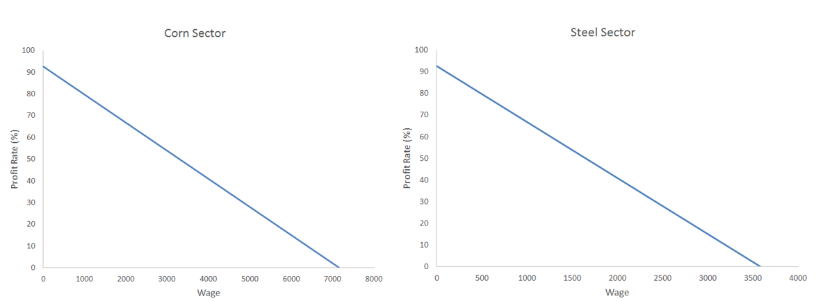
Where does a sector ultimately fall on this line? As emphasized throughout this chapter, heterodox economists understand the determination of the share of the surplus going to owners, managers, workers, and everyone else to ultimately reflect relationships and interactions between people and organizations. Wages may grow relative to profits, moving down the curves in Figure 1, as workers organize and collectively bargain with management, or they may shrink relatively as, for instance, business models move toward employment through independent contracting. Likewise, workers may win pay raises only to find that their employers have clawed them back through price hikes.

The important takeaway here is that, from the heterodox perspective, there is no natural law determining who gets paid how much. Instead, there are only actual people engaged in the historical process of creating, and demanding for themselves a part of, the surplus output.
The similarities between the production possibilities frontier and the wage-profit frontier don’t stop at simply showing a trade-off between the two. As chapter two discussed, the production possibilities frontier is a ‘frontier’ because it is the furthest out that the economy can go, given the current technology and so on. If, for instance, a new invention allowed for more efficient production, the economy could potentially produce beyond the current production possibilities frontier, which would be indicated graphically by a shift outward (up and to the right) of the curve. Similarly, the wage-profit frontier could be increased, allowing for both a higher rate of profits and greater wages, if technological change made it possible to produce more with the same quantities of corn and steel.
What’s different here is that there’s a new constraint on how far out the frontier goes–namely, business spending. That is, as you learned earlier in the chapter, if there are additional unemployed resources to be used (as is often the case in capitalist economies), then the surplus can be expanded simply by businesses deciding to increase their outlays and create that larger surplus. And although wages and profits rates would still ultimately be a matter of power struggles between owners/managers and workers–that is, of how big each slice of the pie will be–the pie itself would be bigger, but only if businesses allow it to grow.
Profits and wages
Thus far, this chapter has emphasized that wages and profits reflect struggles over who will get how much of the surplus, and that ultimately the size of the surplus itself reflects business investment decisions in the aggregate. As you learned in the previous section, this means that, at the macro level of the economy as a whole, investment drives profits, even if profits drive investment at the micro level of the individual business.
Above we’ve argued that an increase in wages must come at the expense of a decrease in profits, given a fixed level of surplus to be had. If workers’ slice of the pie (wages) gets bigger then business owners/managers’ slice (profits) must get smaller, if the pie itself stays the same size. However, there is an additional complication worth noting that recalls, once again, the fact that the way things work at the micro level isn’t always the way things work at the macro level. Specifically, for an individual business, pressing wages down may, all else equal, mean higher profits, but for the economy as a whole this may not be the case.
The reason is that investment isn’t actually the only type of spending ultimately determining the size of the surplus; consumption spending by workers and others (as well as spending by governments and other groups) also impacts how much surplus is produced in the economy. With this in mind, consider the impact of an overall reduction in workers’ wages.
With less money to spend, workers will on the whole consume less, which, if we assume all other spending remains unchanged, will lower total spending. Businesses will see a reduction in sales and respond by reducing output and laying off workers. As a consequence, the surplus will shrink; and even if businesses are enjoying a higher profit rate, a bigger slice of the pie relative to workers, their actual profits may be lower due to the lower total output (that is, a smaller pie).
The same logic could work in reverse, where an increase in wages increases spending by workers, driving businesses to boost output and leading to, well…more pie for everyone.
